
7:00 – 8:00 Research
- Based on the charts from yesterday, I think I’m going to build two matrices to point WEKA at. Essentially, theses matrices will be filled with meta-cluster information
- Average distance from agent to agent. Tightly clustered agents should have low average distances. DBSCAN should also work on this, as well as bootstrapping. That should cover this case:

- Average velocity from agent to agent. I’m not sure what I’ll get from this, but in looking at the explore-explore case and the explore-exploit case, it strikes me that there may be some difference that is meaningful. And in the exploit-exploit case, the velocities should be near zero
 Explore-exploit
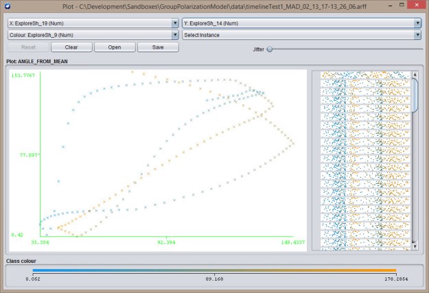 Explore-explore
 - Start with Excel, and then add an ARFF
- Got most of the methods built. Might finish this morning at work.
- Indeed, you can get a lot done when you’re sitting in on a Skype meeting and they’re not talking about your part…
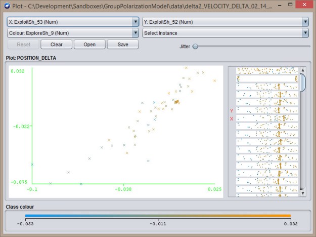
- Ok, so I’ve added comparison matrices as Excel and ARFF output. In this case WEKA does better charting, so here goes. The first chart is exploit-exploit. Note that the majority of points are at 0,0:
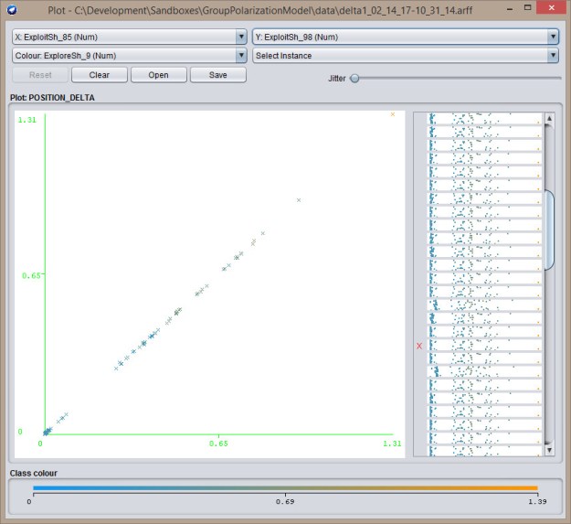 Next, an explore-exploit. In this case, there’s a cluster on the left side of the chart:
 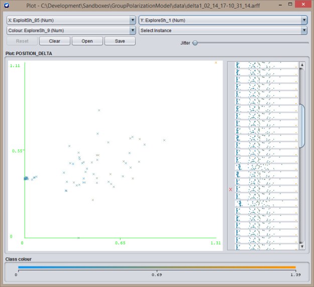 Last, is the explore-explore chart, which has a cluster towards the middle:
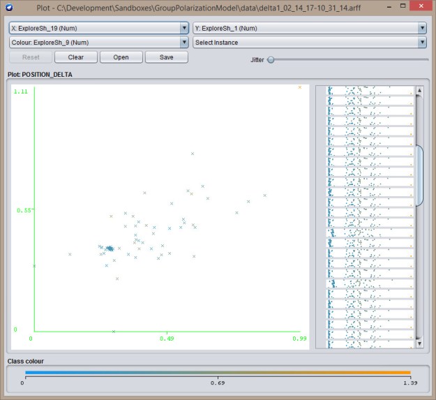
- This data also seems to be good to train a NaiveBayes Classifier. Here’s the result of an initial run:
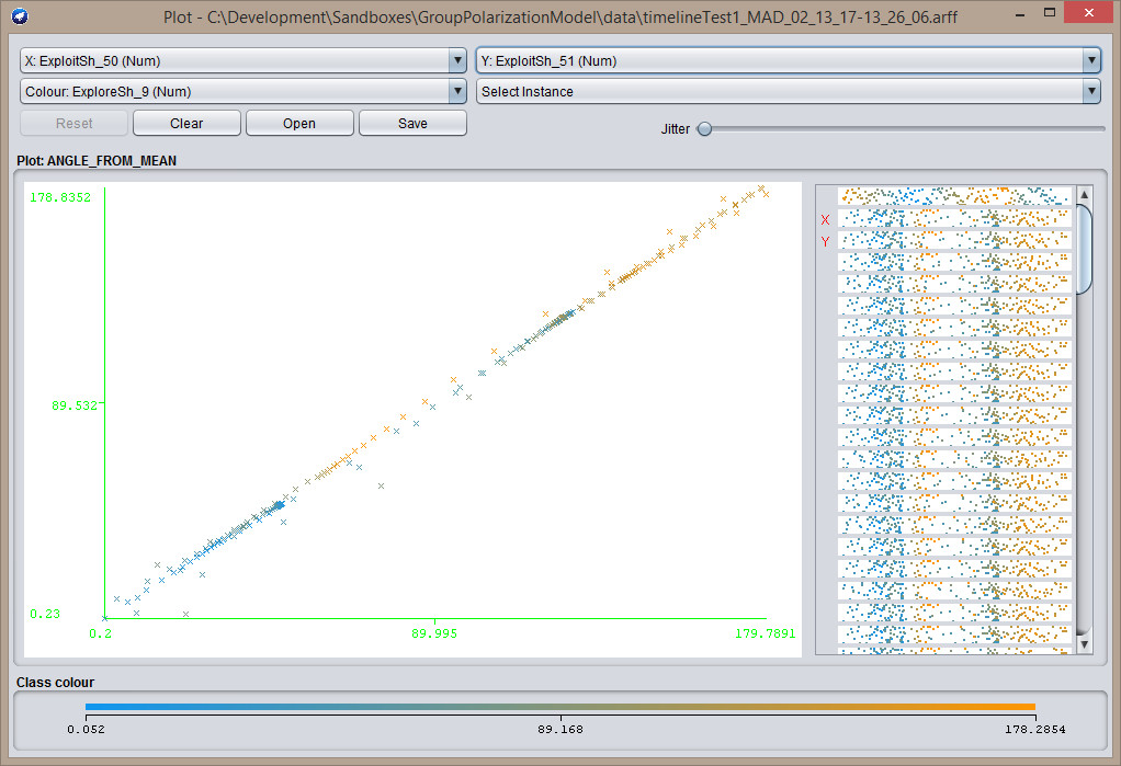
=== Stratified cross-validation === === Summary === Correctly Classified Instances 97 97 % Incorrectly Classified Instances 3 3 % Kappa statistic 0.94 Mean absolute error 0.03 Root mean squared error 0.1732 Relative absolute error 6 % Root relative squared error 34.6337 % Total Number of Instances 100 === Detailed Accuracy By Class === TP Rate FP Rate Precision Recall F-Measure MCC ROC Area PRC Area Class 1.000 0.059 0.942 1.000 0.970 0.942 0.971 0.942 EXPLORER 0.941 0.000 1.000 0.941 0.970 0.942 1.000 1.000 EXPLOITER Weighted Avg. 0.970 0.029 0.972 0.970 0.970 0.942 0.986 0.972 === Confusion Matrix === a b -- classified as 49 0 | a = EXPLORER 3 48 | b = EXPLOITER - Velocity also works, the plots aren’t as crisp, but the classifier accuracy is about the same:
 Exploit-Exploit
  Explore-Exploit
 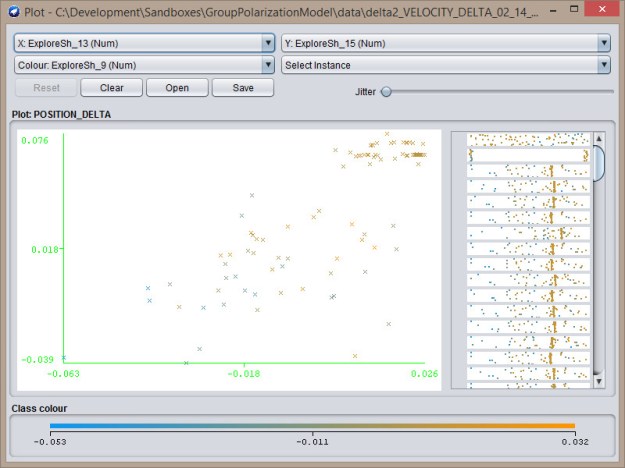 Explore-Explore
 - Again, classification looks good:
=== Stratified cross-validation ===
=== Summary ===

Correctly Classified Instances          99               99      %
Incorrectly Classified Instances         1                1      %
Kappa statistic                          0.98
Mean absolute error                      0.01
Root mean squared error                  0.1
Relative absolute error                  2      %
Root relative squared error             19.9957 %
Total Number of Instances              100

=== Detailed Accuracy By Class ===

                 TP Rate  FP Rate  Precision  Recall   F-Measure  MCC      ROC Area  PRC Area  Class
                 1.000    0.020    0.980      1.000    0.990      0.980    1.000     1.000     EXPLORER
                 0.980    0.000    1.000      0.980    0.990      0.980    1.000     1.000     EXPLOITER
Weighted Avg.    0.990    0.010    0.990      0.990    0.990      0.980    1.000     1.000

=== Confusion Matrix ===

  a  b   -- classified as
 49  0 |  a = EXPLORER
  1 50 |  b = EXPLOITER
- Uploaded new version of the tool to philfeldman.com/GroupPolarization/GroupPloarizationModel.jar
- Average distance from agent to agent. Tightly clustered agents should have low average distances. DBSCAN should also work on this, as well as bootstrapping. That should cover this case:


8:30 – 3:30. BRC
- Either start on the ResearchBrowser or continue with meta-clustering.
- Grooming and sprint planning today – done! And good progress while hanging out on the phone.


You must be logged in to post a comment.