Monthly Archives: January 2017

Phil 1.31.17

Do today

7:00 – 8:00 Research

  • I have a server! tacjour.rs.umbc.edu
  • Starting Filter bubbles, echo chambers, and online news consumption
    • Seth R. Flaxman – I am currently undertaking a postdoc with Yee Whye Teh at Oxford in the computational statistics and machine learning group in the Department of Statistics. My research is on scalable methods and flexible models for spatiotemporal statistics and Bayesian machine learning, applied to public policy and social science areas including crime, emotion, and public health. I helped make a very accessible animation answering the question, What is Machine Learning?
    • Sharad Goel – I’m an Assistant Professor at Stanford in the Department of Management Science & Engineering (in the School of Engineering). I also have courtesy appointments in Sociology and Computer Science. My primary area of research is computational social science, an emerging discipline at the intersection of computer science, statistics, and the social sciences. I’m particularly interested in applying modern computational and statistical techniques to understand and improve public policy.
    • Justin M. Rao – I am a Senior Researcher at Microsoft Research. A member of our New York City lab, an interdisciplinary research group combining social science with computational and theoretical methods, I am currently located at company HQ in the Seattle area, where I am also an Affiliate Professor of Economics at the University of Washington.
    • Spearman’s Rank-Order Correlation
    • Goel, Mason, and Watts (2010) show that a substantial fraction of ties in online social networks are between individuals on opposite sides of the political spectrum, opening up the possibility for diverse content discovery. [p 299]
      • I think this helps in areas where flocking can occur. Changing heading is hardest when opinions are moving in opposite directions. Finding a variety of perspectives may change the dynamic.
    • Specifically, users who predominately visit left-leaning news outlets only very
      rarely read substantive news articles from conservative sites, and vice versa
      for right-leaning readers, an effect that is even more pronounced for opinion
      articles.

      • Is the range of information available from left or right-leaning sites different? Is there another way to look at the populations? I think it’s very easy to get polarized left or right, but seeking diversity is different, and may have a pattern of seeking less polarized voices?
    • Interestingly, exposure to opposing perspectives is higher for the
      channels associated with the highest segregation, search, and social. Thus,
      counterintuitively, we find evidence that recent technological changes both
      increase and decrease various aspects of the partisan divide.

      • To me this follows, because anti belief helps in the polarization process.
    • We select an initial universe of news outlets (i.e., web domains) via the Open Directory Project (ODP, dmoz.org), a collective of tens of thousands of editors who hand-label websites into a classification hierarchy. This gives 7,923 distinct domains labeled as news, politics/news, politics/media, and regional/news. Since the vast majority of these news sites receive relatively little traffic,
      •  Still a good option for mapping. Though I’d like to compare with schema.org
    • Specifically, our primary analysis is based on the subset of users who have read at least ten substantive news articles and at least two opinion pieces in the three-month time frame we consider. This first requirement reduces our initial sample of 1.2 million individuals to 173,450 (14 percent of the total); the second requirement further reduces the sample to 50,383 (4 percent of the total). These numbers are generally lower than past estimates, likely because of our focus on substantive news and opinion (which excludes sports, entertainment, and other soft news), and our explicit activity measures (as opposed to self-reports).
      • Good indicator of explore-exploit in the user population at least in the context of news.
    • We now define the polarity of an individual to be the typical polarity of the news outlet that he or she visits. We then define segregation to be the expected distance between the polarity scores of two randomly selected users. This definition of segregation, which is in line with past work (Dandekar, Goel, and Lee 2013), intuitively captures the idea that segregated populations are those in which pairs of individuals are, on average, far apart.
      • This fits nicely with my notion of belief space
    • ideological-segregation-across-channels
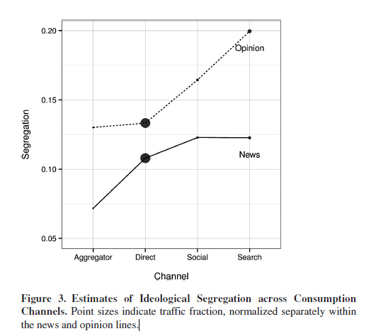
      • This is interesting. Figure 3 shows that aggregators and direct (which have some level of external curation, are substantially less polarized than the social and search-based channels. That’s a good indicator that the visible information horizon makes a difference in what is accessed.
    • our findings do suggest that the relatively recent ability to instantly query large corpora of news articles—vastly expanding users’ choice sets—contributes to increased ideological segregation
      • The frictionlessness of being able to find exactly what you want to see, without being exposed to things that you disagree with.
    • In particular, that level of segregation corresponds to the ideological distance between Fox News and Daily Kos, which represents meaningful differences in coverage (Baum and Groeling 2008) but is within the mainstream political spectrum. Consequently, though the predicted filter bubble and echo chamber mechanisms do appear to increase online segregation, their overall effects at this time are somewhat limited.
      • But this depends on how opinion is moving. We are always redefining normal. It would also be good to look at the news producers using this approach…?
    • This finding of within-user ideological concentration is driven in part by the fact that individuals often simply turn to a single news source for information: 78 percent of users get the majority of their news from a single publication, and 94 percent get a majority from at most two sources. …even when individuals visit a variety of news outlets, they are, by and large, frequenting publications with similar ideological perspectives.
    • opposingpartisanexposure
      • Although I think focussing on ‘opposing’ rather than ‘diverse’ biases these results, this still shows that populations of users behave differently, and that the channel has a distinct effect.
    • …relatively high within-user variation is a product of reading a variety of centrist and right-leaning outlets, and not exposure to truly ideologically diverse content.
      • So left leaning is more diverse across ideology
    • the outlets that dominate partisan news coverage are still relatively mainstream, ranging from the New York Times on the left to Fox News on the right; the more extreme ideological sites (e.g., Breitbart), which presumably benefited from the rise of online publishing, do not appear to qualitatively impact the dynamics of news consumption.

8:30 – 4:00 BRC

  • Finished a second pass through the ResearchBrowser white paper
  • Thinking about optimal sequential clustering
    • A Framework of Mining Semantic Regions from Trajectories
    • This also makes me wonder if we should be looking at our patients as angle from mean
    • Phase 1 : optimize current algorithm to hillclimb for most cluster and least unclustered by varying EPS for a given cluster minimum
    • Phase 2: Do NMF analysis of patient clusters to extract meaningful labels
    • Phase 3: Model patient trajectories through diagnosis space

Phil 1.30.17

7:00 – 8:00 Research

  • Wow, what a weekend. Had to decide whether or not it was better to go to the BWI protest, or finish the abstract, which is an attempt to model and hopefully influence situations like we find ourselves in. Decided to finish the abstract. Hopefully that’s the right choice.
  • Working on trying to figure out why I can’t classify in WEKA any more.
    • Installing the latest and greatest (3.8.1)
    • Using this data: anglefrommeanchart
    • Yay! So you don’t have to do a lot of preprocessing to classify in WEKA.
      • Read in the training data under the ‘Preprocess’ tab
      • Switch to the ‘Classify’ tab
      • (In this case) select NaiveBayes, and what to classify against – AgentBias
      • Build the model using cross-validation
      • Load the test model, selecting AgentBias to classify against
      • Then right-click and select re-evaluate model on current test set wekasuppliedtest
      • Run the tests! Here’s a screenshot of classifier errors when using mean angle stats (BIG signal) Thatclassifiererrorsmeanangle
      • That is a beautiful thing. The chart shows the variance of each agent for the duration of the run with respect to the direction cosine.  Polarized agents (red) have a low variance and ‘explorer’ agents (blue) have a high variance. Here’s the raw output
        === Run information ===
        
        Scheme:       weka.classifiers.misc.InputMappedClassifier -I -trim -W weka.classifiers.bayes.NaiveBayes
        Relation:     ANGLE_FROM_MEAN_STATS
        Instances:    200
        Attributes:   7
                      name_
                      AgentBias_
                      Mean
                      Fifth
                      Fiftieth
                      NintyFifth
                      Variance
        Test mode:    user supplied test set:  size unknown (reading incrementally)
        
        === Classifier model (full training set) ===
        
        InputMappedClassifier:
        
        Naive Bayes Classifier
        
                           Class
        Attribute       EXPLORER EXPLOITER
                           (0.5)     (0.5)
        ===================================
        name_
          shape_0             2.0       1.0
          shape_1             2.0       1.0
          shape_10            2.0       1.0
          shape_100           1.0       2.0
          shape_101           1.0       2.0
          shape_102           1.0       2.0
          shape_103           1.0       2.0
          shape_104           1.0       2.0
          shape_105           1.0       2.0
          shape_106           1.0       2.0
          shape_107           1.0       2.0
          shape_108           1.0       2.0
          shape_109           1.0       2.0
          shape_11            2.0       1.0
          shape_110           1.0       2.0
          shape_111           1.0       2.0
          shape_112           1.0       2.0
          shape_113           1.0       2.0
          shape_114           1.0       2.0
          shape_115           1.0       2.0
          shape_116           1.0       2.0
          shape_117           1.0       2.0
          shape_118           1.0       2.0
          shape_119           1.0       2.0
          shape_12            2.0       1.0
          shape_120           1.0       2.0
          shape_121           1.0       2.0
          shape_122           1.0       2.0
          shape_123           1.0       2.0
          shape_124           1.0       2.0
          shape_125           1.0       2.0
          shape_126           1.0       2.0
          shape_127           1.0       2.0
          shape_128           1.0       2.0
          shape_129           1.0       2.0
          shape_13            2.0       1.0
          shape_130           1.0       2.0
          shape_131           1.0       2.0
          shape_132           1.0       2.0
          shape_133           1.0       2.0
          shape_134           1.0       2.0
          shape_135           1.0       2.0
          shape_136           1.0       2.0
          shape_137           1.0       2.0
          shape_138           1.0       2.0
          shape_139           1.0       2.0
          shape_14            2.0       1.0
          shape_140           1.0       2.0
          shape_141           1.0       2.0
          shape_142           1.0       2.0
          shape_143           1.0       2.0
          shape_144           1.0       2.0
          shape_145           1.0       2.0
          shape_146           1.0       2.0
          shape_147           1.0       2.0
          shape_148           1.0       2.0
          shape_149           1.0       2.0
          shape_15            2.0       1.0
          shape_150           1.0       2.0
          shape_151           1.0       2.0
          shape_152           1.0       2.0
          shape_153           1.0       2.0
          shape_154           1.0       2.0
          shape_155           1.0       2.0
          shape_156           1.0       2.0
          shape_157           1.0       2.0
          shape_158           1.0       2.0
          shape_159           1.0       2.0
          shape_16            2.0       1.0
          shape_160           1.0       2.0
          shape_161           1.0       2.0
          shape_162           1.0       2.0
          shape_163           1.0       2.0
          shape_164           1.0       2.0
          shape_165           1.0       2.0
          shape_166           1.0       2.0
          shape_167           1.0       2.0
          shape_168           1.0       2.0
          shape_169           1.0       2.0
          shape_17            2.0       1.0
          shape_170           1.0       2.0
          shape_171           1.0       2.0
          shape_172           1.0       2.0
          shape_173           1.0       2.0
          shape_174           1.0       2.0
          shape_175           1.0       2.0
          shape_176           1.0       2.0
          shape_177           1.0       2.0
          shape_178           1.0       2.0
          shape_179           1.0       2.0
          shape_18            2.0       1.0
          shape_180           1.0       2.0
          shape_181           1.0       2.0
          shape_182           1.0       2.0
          shape_183           1.0       2.0
          shape_184           1.0       2.0
          shape_185           1.0       2.0
          shape_186           1.0       2.0
          shape_187           1.0       2.0
          shape_188           1.0       2.0
          shape_189           1.0       2.0
          shape_19            2.0       1.0
          shape_190           1.0       2.0
          shape_191           1.0       2.0
          shape_192           1.0       2.0
          shape_193           1.0       2.0
          shape_194           1.0       2.0
          shape_195           1.0       2.0
          shape_196           1.0       2.0
          shape_197           1.0       2.0
          shape_198           1.0       2.0
          shape_199           1.0       2.0
          shape_2             2.0       1.0
          shape_20            2.0       1.0
          shape_21            2.0       1.0
          shape_22            2.0       1.0
          shape_23            2.0       1.0
          shape_24            2.0       1.0
          shape_25            2.0       1.0
          shape_26            2.0       1.0
          shape_27            2.0       1.0
          shape_28            2.0       1.0
          shape_29            2.0       1.0
          shape_3             2.0       1.0
          shape_30            2.0       1.0
          shape_31            2.0       1.0
          shape_32            2.0       1.0
          shape_33            2.0       1.0
          shape_34            2.0       1.0
          shape_35            2.0       1.0
          shape_36            2.0       1.0
          shape_37            2.0       1.0
          shape_38            2.0       1.0
          shape_39            2.0       1.0
          shape_4             2.0       1.0
          shape_40            2.0       1.0
          shape_41            2.0       1.0
          shape_42            2.0       1.0
          shape_43            2.0       1.0
          shape_44            2.0       1.0
          shape_45            2.0       1.0
          shape_46            2.0       1.0
          shape_47            2.0       1.0
          shape_48            2.0       1.0
          shape_49            2.0       1.0
          shape_5             2.0       1.0
          shape_50            2.0       1.0
          shape_51            2.0       1.0
          shape_52            2.0       1.0
          shape_53            2.0       1.0
          shape_54            2.0       1.0
          shape_55            2.0       1.0
          shape_56            2.0       1.0
          shape_57            2.0       1.0
          shape_58            2.0       1.0
          shape_59            2.0       1.0
          shape_6             2.0       1.0
          shape_60            2.0       1.0
          shape_61            2.0       1.0
          shape_62            2.0       1.0
          shape_63            2.0       1.0
          shape_64            2.0       1.0
          shape_65            2.0       1.0
          shape_66            2.0       1.0
          shape_67            2.0       1.0
          shape_68            2.0       1.0
          shape_69            2.0       1.0
          shape_7             2.0       1.0
          shape_70            2.0       1.0
          shape_71            2.0       1.0
          shape_72            2.0       1.0
          shape_73            2.0       1.0
          shape_74            2.0       1.0
          shape_75            2.0       1.0
          shape_76            2.0       1.0
          shape_77            2.0       1.0
          shape_78            2.0       1.0
          shape_79            2.0       1.0
          shape_8             2.0       1.0
          shape_80            2.0       1.0
          shape_81            2.0       1.0
          shape_82            2.0       1.0
          shape_83            2.0       1.0
          shape_84            2.0       1.0
          shape_85            2.0       1.0
          shape_86            2.0       1.0
          shape_87            2.0       1.0
          shape_88            2.0       1.0
          shape_89            2.0       1.0
          shape_9             2.0       1.0
          shape_90            2.0       1.0
          shape_91            2.0       1.0
          shape_92            2.0       1.0
          shape_93            2.0       1.0
          shape_94            2.0       1.0
          shape_95            2.0       1.0
          shape_96            2.0       1.0
          shape_97            2.0       1.0
          shape_98            2.0       1.0
          shape_99            2.0       1.0
          [total]           300.0     300.0
        
        Mean
          mean             84.763     5.237
          std. dev.       27.2068    0.7459
          weight sum          100       100
          precision        0.6792    0.6792
        
        Fifth
          mean            15.0052    0.3847
          std. dev.       15.1486    0.1425
          weight sum          100       100
          precision        0.3966    0.3966
        
        Fiftieth
          mean                  0         0
          std. dev.        0.0017    0.0017
          weight sum          100       100
          precision          0.01      0.01
        
        NintyFifth
          mean           162.5673   23.0501
          std. dev.       18.6542    2.4072
          weight sum          100       100
          precision        0.7954    0.7954
        
        Variance
          mean           147.5186   22.7738
          std. dev.       20.0571    2.3901
          weight sum          100       100
          precision        0.7627    0.7627
        
        
        Attribute mappings:
        
        Model attributes      	    Incoming attributes
        ----------------------	    ----------------
        (nominal) name_       	--> 1 (nominal) name_
        (nominal) AgentBias_  	--> 2 (nominal) AgentBias_
        (numeric) Mean        	--> 3 (numeric) Mean
        (numeric) Fifth       	--> 4 (numeric) Fifth
        (numeric) Fiftieth    	--> 5 (numeric) Fiftieth
        (numeric) NintyFifth  	--> 6 (numeric) NintyFifth
        (numeric) Variance    	--> 7 (numeric) Variance
        
        
        Time taken to build model: 0 seconds
        
        === Evaluation on test set ===
        
        Time taken to test model on supplied test set: 0 seconds
        
        === Summary ===
        
        Correctly Classified Instances         100              100      %
        Incorrectly Classified Instances         0                0      %
        Kappa statistic                          1     
        Mean absolute error                      0     
        Root mean squared error                  0     
        Relative absolute error                  0      %
        Root relative squared error              0      %
        Total Number of Instances              100     
        
        === Detailed Accuracy By Class ===
        
                         TP Rate  FP Rate  Precision  Recall   F-Measure  MCC      ROC Area  PRC Area  Class
                         1.000    0.000    1.000      1.000    1.000      1.000    1.000     1.000     EXPLORER
                         1.000    0.000    1.000      1.000    1.000      1.000    1.000     1.000     EXPLOITER
        Weighted Avg.    1.000    0.000    1.000      1.000    1.000      1.000    1.000     1.000     
        
        === Confusion Matrix ===
        
          a  b   -- classified as
         50  0 |  a = EXPLORER
          0 50 |  b = EXPLOITER

8:30 – 2:30 BRC

  • Working on white paper

Phil 1.27.17

7:45 – 8:30 Research

  • Working on the abstract
  • Changed the sim code so that it doesn’t have to do a new fun for each ARFF file
  • I seem to have forgotten how to compare two data sets. This video seems to have the answer. Made some new data files. Try it on the weekend?

9:00 – 5:30 BRC

  • Working on paper
  • Meeting with Aaron, Gregg, Nir, Theresa

Phil 1.26.17

7:00 – 11:00 Research

11:30 – 4:30 BRC

  • Some problem updating the CSE blacklists. Fixed
  • Started white paper on Unstructured text analysis. Due tomorrow.
  • Curating on production now.

Phil 1.25.17

7:00 – 8:00 Research

  • Got news that my server at UMBC has a ticket for its creation. Woohoo!
  • Got batch processing running for the flocking app. Need to analyze the output to find the best output form for detecting differences
    • I think that comparing headings could work too. There are two things to look at
      • The average heading vector. if it’s large, everyone is aligned if it’s zero, then it’s either random or the agents are orbiting
      • The comparison of the individual agent to the average vector. This should ideally take into account the size of the average vector.
    • Also still thinking about some way to classify agents without dimension reduction. This paper might help: Bayesian Chain Classifiers for Multidimensional Classification (JH Zaragoza, LE Sucar, EF Morales, C Bielza… – IJCAI, 2011)
  • Working on abstract
  • Need to get rid of the sum object and do descriptive stats: mean, variance, etc. Train on these.

8:30 – 5:00 BRC

  • Several tasks for decoupling CSEs from BRC
  • More curating
  • More blacklisting

Phil 1.24.17

7:00 – 8:00 Research

  • Getting CHI review out of the way. Done!
  • Back to extended abstract

8:30 – 5:00

  • Got the batch processing done and ran a test. Need to send through WEKA
  • Curated

Phil 1.23.17

7:00 – 8:00 Research

  • Write CHI review today!
  • Started writing abstract by going through The Law of Group Polarization and pulling out relevant quotes that describe what the model should do. Also found a couple of well-cited papers on flocking as group decision making. Still need to dig up sociophysics citations on:
    • Multidimensional voter models(?)
    • Reynolds flocking algorithm
    • Polarization as a static result.
  • Decision-making processes: The case of collective movements
  • Do I need to change the “allow interaction” from binary to continuous (basically a weight on the interaction value?  The amount of “isolation” could then be varied.

8:30 – 5:30 BRC

  • Fixing the parser for XmlLoader dates – done
  • Built the batch state machine
  • Ran a sim from file!
  • Need to
  • Fixed an error where I put a set of .com pages in the search instead of exclude file.
  • Curating
  • Sprint review

Phil 1.20.17

7:00 – 7:45 Research

9:30 – 5:00 BRC

  • Updated all the CSEs
  • Working through loading of config files. Far too fancy, but killing time before the review. Which has been delayed to 2:00. With technical difficulties, 2:?? Canceled.
  • For the review, read in integrity1.xlsx. It’s small enough to load reasonably quickly
  • Loading config files!

Phil 1.19.17

7:00 – 8:00 Research

8:30 – 3:30 BRC

  • Updated Java, recompiled and verified everything
  • Working on classifying clusters
    • Adding multiple config loads
    • Need to add a “settling time” before recording starts automatically

Phil 1.18.177

7:00 – 8:00, 8:30 – 3:30 Research

  • Working title Interpreting ‘The Law of Group Polarization” with flocking behavior
    • Multidimensional exposes information distance and diversity issues (low dimensions = easier flocking, and the converse)
    • Reynolds-style flocking behavior means that agreement is not a static value, but changes. This brings up questions about how to identify GP, particularly in high dimensions
    • Adjusting social horizons results in three states (Phase change)
      • Random
      • Flocking
      • Polarized Group
    • The impact of visible diversity of GP.
    • Machine learning for identification of states/types
  • Wired up RunConfig to support border types
  • Closing the loop with Tim Champ for server space at UMBC
  • Downloaded the format and created a CollectiveIntelligence 2017 folder. Looking back through the 2015 conference, there were visible abstracts. Going to read a few to get a sense.
  • Uploaded the executable jar https://philfeldman.com/GroupPolarization/GroupPolarizationModel.jar
  • Adding ARFF output – done! First try:
    === Stratified cross-validation ===
    === Summary ===
    
    Correctly Classified Instances          98               98      %
    Incorrectly Classified Instances         2                2      %
    Kappa statistic                          0.898 
    Mean absolute error                      0.02  
    Root mean squared error                  0.1414
    Relative absolute error                 10.6977 %
    Root relative squared error             47.1207 %
    Total Number of Instances              100     
    
    === Detailed Accuracy By Class ===
    
                     TP Rate  FP Rate  Precision  Recall   F-Measure  MCC      ROC Area  PRC Area  Class
                     1.000    0.022    0.833      1.000    0.909      0.903    0.989     0.833     EXPLORER
                     0.978    0.000    1.000      0.978    0.989      0.903    0.989     0.998     EXPLOITER
    Weighted Avg.    0.980    0.002    0.983      0.980    0.981      0.903    0.989     0.981     
    
    === Confusion Matrix ===
    
      a  b   
     10  0 |  a = EXPLORER
      2 88 |  b = EXPLOITER
  • One run vs another, using average angle difference:
    === Summary ===
    
    Correctly Classified Instances          96               96      %
    Incorrectly Classified Instances         4                4      %
    Kappa statistic                          0.8837
    Mean absolute error                      0.04  
    Root mean squared error                  0.2   
    Relative absolute error                 12.3636 %
    Root relative squared error             49.9946 %
    Total Number of Instances              100     
    
    === Detailed Accuracy By Class ===
    
                     TP Rate  FP Rate  Precision  Recall   F-Measure  MCC      ROC Area  PRC Area  Class
                     1.000    0.050    0.833      1.000    0.909      0.890    0.975     0.833     EXPLORER
                     0.950    0.000    1.000      0.950    0.974      0.890    0.994     0.998     EXPLOITER
    Weighted Avg.    0.960    0.010    0.967      0.960    0.961      0.890    0.990     0.965     
    
    === Confusion Matrix ===
    
      a  b   -- classified as
     20  0 |  a = EXPLORER
      4 76 |  b = EXPLOITER
  • Need a checkbox for cross-bias interaction. Done! Now I can train against two populations with and without interactions
  • Spreadsheet with new tabs and some nifty charts: meanangletest_01_18_17-14_07_32

3:30 – 4:30

  • Walked through scoring issues with Aaron
  • Realized that the above work can be used for classifying clusters with ML.

Phil 1.17.17

Shower thought for today: The social horizon for flocking to occur is sqrt(dimensions)*k. This means the lower the number of dimensions, the easier to flock, while higher dimensions (i.e. more diverse) make flocking harder. Conversely, by watching the flocking behavior of individuals, it may be possible to infer the number of dimensions they are paying attention to.

Collective intelligence conference. Abstracts are 4 pages. Format is here, and here’s the program with abstracts from 2016. Need to dig up a password

7:00 – 8:00 Research

  • Procrastinating about writing. I think I want to have some of the different border conditions in place to see if there is any effect.
  • Made a ACTIVE, INACTIVE and DORMANT state.
    • ACTIVE is moves and is visible
    • INACTIVE is not visible, effectively removed from all interaction. Hitting a lethal boundary sets state to INACTIVE
    • DORMANT is visible, but not active
    • Added the combo and config
    • Set behavior so that moving requires an ACTIVE state and visibility requires a non INACTIVE state
    • Need to wire up border behaviors and set colors for DORMANT (gray) and INACTIVE (black)
  • Fixed the bug where a re-initialized run was repeating the same data.

8:30 – 5:00 BRC

  • Working on documentation. Done!
  • Made a few changes to NMFGui to improve saving and parsing .

Phil 1.16.17

7:00 – 8:00 Research

  •  Walls
    • infinite
    • fatal
    • force at a radius
    • toroidal with distribution across the torus
  • Look for data sets
    Sentiment analysis flocking on a twitter subject
  • Add ‘samples’ indicator – done
  • Add some kind of live/dead state for lethal walls
  • Tried recording a 10D run and had to reset. Recorded the same item for the entire run.
  • Isolating and weighting are broken. Need to fix.

8:30 – 5:00 BRC

  • Cleaning up IntegrityMatrixBuilder enough so that it can be checked in. Done
  • Working on documentation. Worried about scope creep and having to document EVERYTHING
  • My openVPN is denied again, so can’t connect to the remote DB?
  • Built new clusters on Aaron’s machine

Phil 1.15.17

  • Make sure that distance calculations are double buffered. I think this can be done bay have a ‘cur’ and ‘previous’ ParticleBelief
    • Added prevBelief and curBelief.
    • added deepUpdate() method to ParticleBelief
    • No change. Yay!
  •  Walls
    • infinite
    • fatal
    • force at a radius
    • toroidal with distribution across the torus
  • Look for data sets
    Sentiment analysis flocking on a twitter subject
  • Add ‘samples’ indicator
  • Add some kind of live/dead state for lethal walls

Phil 1.13.17

7:00 – 8:30 Research

  • First research runs
  • All Exploit
    • No group visibility (NGV R = 0)
    • Partial group visibility (PGV R = 0.1 )
    • Partial group visibility (PGV R = 0.2 )
    • Partial group visibility (PGV R = 0.4 )
    • Partial group visibility (PGV R = 0.8 )
    • Full group visibility (FGV R = 10.0)(
  • 10% Explore (NGV R = 0) / 90% Exploit
    • Exploit (PGV R = 0.1 )
    • Exploit (PGV R = 0.2 )
    • Exploit (PGV R = 0.4 )
    • Exploit (PGV R = 0.4 )
    • Exploit (FGV R = 10.0 )

9:00 – 3:30 BRC

  • Created mbrnum_cluster.csv for Bob to look at
  • Spent the rest of the day fixing the csv file. mbrnum should have been mmberrow, no spaces, etc.
  • Tried a rollup of diagnosis codes, which produced more clusters. Using that as a first pass

4:00 – 5:00 Meeting with Don

  • Make sure that distance calculations are double buffered. I think this can be done bay have a ‘cur’ and ‘previous’ statementList inside of ParticleBelief.
  •  Walls
    • infinite
    • fatal
    • force at a radius
    • toroidal with distribution across the torus
  • Look for data sets
    Sentiment analysis flocking on a twitter subject

Phil 1.12.17

7:00 – 8:30 Research

  • Set up page that shows the 5th, 50th and 95th percentiles for each statement’s population sample. Put in a new tab.
  • Add a tab that shows the 5th/95th – the 50th? That could sum to a nice chart
  • The above two items will need a Collection of Percentiles for all agents positions at a step across all dimensions. Done. Charts look cool, too. Will generate data tomorrow and load up the laptop for chat with Don. echochambertest

9:00 – 5:00 BRC