Phil 3.2.17

7:00 – 8:00 Research

  • Scheduled a meeting with Don for Monday at 4:00
  • Working on finding submission formats for my top 3
    • Physical Review E
      • Author page
      • Here’s the format
        • My guess is that there will have to be equations for neighbor calculation (construct a vector from visible neighbors and slew heading and speed) plus maybe a table for the figure 8? Not sure how to do that since the populations had no overlap.
      • Length FAQ Looks like 4500 words
        Rapid Communication 4500 words
        Comment / Reply 3500 words
      • Include:
        • Any text in the body of the article
        • Any text in a figure caption or table caption
        • Any text in a footnote or an endnote
        • I’m at 3073 words in the content.
        • Here’s the figure word eqivalents:
          figure xsize ysize aspect one col two cols
          10 6.69 4.03 1.66 110.26 401.04
          9 8.13 2.85 2.85 72.56 250.24
          8 6.28 5.14 1.22 142.79 531.14
          7 8.78 2.94 2.98 70.31 241.23
          6 6.64 3.97 1.67 109.74 398.97
          5 6.80 3.89 1.75 105.79 383.15
          4 8.13 2.85 2.85 72.56 250.24
          3 8.13 2.85 2.85 72.56 250.24
          2 8.13 2.85 2.85 72.56 250.24
          1 7.26 5.44 1.33 132.40 489.59
          961.52 3446.08
        • So it looks like the word count is between 4,034 and 6,519
      • IEEE Transactions on Automatic Control
        • Instructions for full papers
          • PDF
          • Manuscript style is in section C. References are like ACM
          • Normally 12 pages and no more than 16
          • A mandatory page charge is imposed on all accepted full papers exceeding 12 Transactions formatted pages including illustrations, biographies and photos . The charge is $125 per page for each page over the first 12 pages and is a prerequisite for publication. A maximum of 4 such additional pages (for a total of 16 pages) is allowed. 
          • Note that the authors will be asked to submit a single-column double-spaced version of their paper as well, under Supplementary Materials
          • To enhance the appearance of your paper on IEEEXplore®, a Graphical Abstract can be displayed along with traditional text. The Graphical Abstract should provide a clear, visual summary of your paper’s findings by means of an image, animation, video, or audio clip. NOTE: The graphical abstract is considered a part of the technical content of the paper, and you must provide it for peer review during the paper submission process.
        • Submission policy
        • MSWord template and Instructions on How to Create Your Paper
        • Guidelines for graphics and charts
      • Journal of Political Philosophy (Not sure if it makes sense, but this was where The Law of Group Polarization was published)
        • Author Guidelines 
        • Manuscripts accepted for publication must be put into JPP house style, as follows:
          • SPELLING AND PUNCTUATION: Authors may employ either American or English forms, provided that style is used consistently throughout their submission.
          • FOOTNOTES: Should be numbered consecutively. Authors may either:
            • employ footnotes of the traditional sort, containing all bibliographic information within them; or else
            • collect all bibliographic information into a reference list at the end of the article, to which readers should be referred by footnotes (NOT in-text reference) of the form ‘Barry 1965, p. 87’.
          • BIBLIOGRAPHIC INFORMATION: should be presented in either of the following formats:
            • If incorporated into the footnotes themselves:
              Jürgen Habermas, Legitimation Crisis, trans. Thomas McCarthy (London: Heinemann, 1976), p. 68.
              Louise Antony, ‘The socialization of epistemology’, Oxford Handbook of Contextual Political Analysis, ed. by Robert E. Goodin and Charles Tilly (Oxford: Oxford University Press, 2006, pp.58-77, at p. 62.
              John Rawls ‘Justice as fairness’, Philosophical Review, 67 (1958), 164-94 at p. 185.
            • If collected together in a reference list at the end of the article:
              Habermas, Jurgen. 1976. Legitimation Crisis, trans. Thomas McCarthy. London: Heinemann.
              Antony, Louise. 2006. The socialization of epistemology. Pp. 58-77 in Oxford Handbook of Contextual Political Analysis, ed. by Robert E. Goodin and Charles Tilly. Oxford: Oxford University Press.
              Rawls, John. 1958. Justice as Fairness. Philosophical Review, 67, 164-94.
            • In footnotes/references, spelling should follow the original while punctuation should conform to the style adopted in the body of the text, being either American (double quotation marks outside closing commas and full stops) or English (single quotation marks inside them).For Survey Articles or Debates, option (ii) – i.e., the reference list at the end of the article, together with the corresponding footnote style – is preferred.
        • Nature (Yeah, I know. But as a letter?)
          • Letters are 4 pages, articles are 5
          • ‘For authors’ site map
          • Presubmission enquiries are not required for Articles or Letters, and can be difficult to assess reliably; Nature editors cannot make an absolute commitment to have a contribution refereed before seeing the entire paper.
          • Editorial process
          • Letters
            • Letters are short reports of original research focused on an outstanding finding whose importance means that it will be of interest to scientists in other fields.

              They do not normally exceed 4 pages of Nature, and have no more than 30 references. They begin with a fully referenced paragraph, ideally of about 200 words, but certainly no more than 300 words, aimed at readers in other disciplines. This paragraph starts with a 2-3 sentence basic introduction to the field; followed by a one-sentence statement of the main conclusions starting ‘Here we show’ or equivalent phrase; and finally, 2-3 sentences putting the main findings into general context so it is clear how the results described in the paper have moved the field forwards.

              Please refer to our annotated example to see how the summary paragraph for a Letter should be constructed.

              The rest of the text is typically about 1,500 words long. Any discussion at the end of the text should be as succinct as possible, not repeating previous summary/introduction material, to briefly convey the general relevance of the work.

              Letters typically have 3 or 4 small display items (figures or tables).

              Word counts refer to the text of the paper. References, title, author list and acknowledgements do not have to be included in total word counts

8:30 – 5:30 BRC

  • Just read Gregg’s response to the white paper. He seems to think that TF is just deep NN. Odd
  • Working through fully_connected_feed.py from the TF Mechanics 101 tutorial
  • Multiple returns works in python:
    def placeholder_inputs(batch_size):
        images_placeholder = tf.placeholder(tf.float32, shape=(batch_size,
                                                               Mnist.IMAGE_PIXELS))
        labels_placeholder = tf.placeholder(tf.int32, shape=(batch_size))
        return images_placeholder, labels_placeholder
    
    images_placeholder, labels_placeholder = placeholder_inputs(FLAGS.batch_size)
  • The logit (/ˈlɪt/ loh-jit) function is the inverse of the sigmoidal “logistic” function or logistic transform used in mathematics, especially in statistics. When the function’s parameter represents a probability p, the logit function gives the log-odds, or the logarithm of the odds p/(1 − p).[1]
  • In this case,
    logits =  Tensor("softmax_linear/add:0", shape=(100, 10), dtype=float32)
  • Here are some of the other variables:
    images_placeholder =  Tensor("Placeholder:0", shape=(100, 784), dtype=float32)
    labels_placeholder =  Tensor("Placeholder_1:0", shape=(100,), dtype=int32)
    logits =  Tensor("softmax_linear/add:0", shape=(100, 10), dtype=float32)
    loss =  Tensor("xentropy_mean:0", shape=(), dtype=float32)
    train_op =  name: "GradientDescent"
    op: "AssignAdd"
    input: "global_step"
    input: "GradientDescent/value"
    attr {
      key: "T"
      value {
        type: DT_INT32
      }
    }
    attr {
      key: "_class"
      value {
        list {
          s: "loc:@global_step"
        }
      }
    }
    attr {
      key: "use_locking"
      value {
        b: false
      }
    }
    
    eval_correct =  Tensor("Sum:0", shape=(), dtype=int32)
    summary =  Tensor("Merge/MergeSummary:0", shape=(), dtype=string)
  • Note that everything is a Tensor except the train_op, which is declared as follows
    # Add to the Graph the Ops that calculate and apply gradients.
    train_op = Mnist.training(loss, FLAGS.learning_rate)
    print("train_op = ", train_op)
  • It looks like dictionaries are the equivalent of may labeled matrices
    def fill_feed_dict(data_set, images_pl, labels_pl):
        """Fills the feed_dict for training the given step.
        A feed_dict takes the form of:
        feed_dict = {
            : ,
            ....
        }
        Args:
          data_set: The set of images and labels, from input_data.read_data_sets()
          images_pl: The images placeholder, from placeholder_inputs().
          labels_pl: The labels placeholder, from placeholder_inputs().
        Returns:
          feed_dict: The feed dictionary mapping from placeholders to values.
        """
        # Create the feed_dict for the placeholders filled with the next
        # `batch size` examples.
        images_feed, labels_feed = data_set.next_batch(FLAGS.batch_size,
                                                       FLAGS.fake_data)
        feed_dict = {
            images_pl: images_feed,
            labels_pl: labels_feed,
        }
        return feed_dict
  • lookup_ops seems to have the pieces we want. Now I just have to make it run…

Training?

Last-second proposal writing

Aaron 3.1.17

  • TensorFlow
    • Figuring out TensorFlow documentation and tutorials (with a focus on matrix operations, loading from hadoop, and clustering).
    • Really basic examples with tiny data sets like linear regression with gradient descent optimizers are EASY. Sessions, variables, placeholders, and other core artifacts all make sense. Across the room Phil’s hair is getting increasingly frizzy as he’s dealing with more complicated examples that are far less straightforward.
  • Test extraction of Hadoop records
    • Create TF tensors using Python against HBASE tables to see if the result is performant enough (otherwise recommend we write a MapReduce job to build out a proto file consumed by TF)
  • Test polar coordinates against client data
    • See if we can use k-means/DBSCAN against polar coordinates to generate the correct clusters with known data). If we cannot use polar coordinates for dimension reduction, what process is required to implement DBSCAN in TensorFlow?
  • Architecture Diagram
    • The artifacts for this sprint’s completion are architecture diagrams and proposal for next sprint’s implementation. I haven’t gotten feedback from the customer about our proposed framework, but it will come up in our end-of-sprint activities. Design path and flow diagram are due on Wednesday.
  • Cycling
    • I did my first 15.2 mile ride today. My everything hurts, and my average speed was way down from yesterday, but I finished.

Phil 3.1.17

It’s March and no new wars! Hooray!

7:00 – 8:00 Research

8:30 – 4:30 BRC

  • More TensorFlow
    • MNIST tutorial – clear, but a LOT of stuff
    • Neural Networks and Deep Learning is an online book referenced in the TF documentation (at least the softmax chapter)
    • A one-hot vector is a vector which is 0 in most dimensions, and 1 in a single dimension. In this case, the nth digit will be represented as a vector which is 1 in the nth dimension. For example, 3 would be [0,0,0,1,0,0,0,0,0,0]. Consequently, mnist.train.labels is a [55000, 10] array of floats.
    • If you want to assign probabilities to an object being one of several different things, softmax is the thing to do, because softmax gives us a list of values between 0 and 1 that add up to 1. Even later on, when we train more sophisticated models, the final step will be a layer of softmax.
    • x = tf.placeholder(tf.float32, [None, 784])

      We represent this as a 2-D tensor of floating-point numbers, with a shape [None, 784]. (Here None means that a dimension can be of any length.)

    • A good explanation of cross-entropy, apparently.
    • tf.reduce_mean
    • Success!!! Here’s the code:
      import tensorflow as tf
      from tensorflow.examples.tutorials.mnist import input_data
      
      mnist = input_data.read_data_sets("MNIST_data/", one_hot=True)
      
      x = tf.placeholder(tf.float32, [None, 784])
      
      W = tf.Variable(tf.zeros([784, 10]))
      b = tf.Variable(tf.zeros([10]))
      
      y = tf.nn.softmax(tf.matmul(x, W) + b)
      
      y_ = tf.placeholder(tf.float32, [None, 10]) #note that y_ means 'y prme'
      
      cross_entropy = tf.reduce_mean(-tf.reduce_sum(y_ * tf.log(y), reduction_indices=[1]))
      
      train_step = tf.train.GradientDescentOptimizer(0.5).minimize(cross_entropy)
      
      sess = tf.InteractiveSession()
      
      tf.global_variables_initializer().run()
      
      for _ in range(1000):
          batch_xs, batch_ys = mnist.train.next_batch(100)
          sess.run(train_step, feed_dict={x: batch_xs, y_: batch_ys})
      
      correct_prediction = tf.equal(tf.argmax(y,1), tf.argmax(y_,1))
      accuracy = tf.reduce_mean(tf.cast(correct_prediction, tf.float32))
      print(sess.run(accuracy, feed_dict={x: mnist.test.images, y_: mnist.test.labels}))
    • And here are the results:
      C:\Users\philip.feldman\AppData\Local\Programs\Python\Python35\python.exe C:/Development/Sandboxes/TensorflowPlayground/HelloPackage/MNIST_tutorial.py
      Extracting MNIST_data/train-images-idx3-ubyte.gz
      Extracting MNIST_data/train-labels-idx1-ubyte.gz
      Extracting MNIST_data/t10k-images-idx3-ubyte.gz
      Extracting MNIST_data/t10k-labels-idx1-ubyte.gz
      
      0.9192
    • Working on the advanced tutorial. Fixed fully_connected_feed.py to work with local data.
    • And then my brain died

Aaron 2.28.17

9:00 – BRC

  • TensorFlow
    • Installed following TF installation guide.
    • Found issues with the install instructions almost immediately. Found this link  with a suggestion that I followed to get it installed.
    • Almost immediately found that the Hello World example succeeded with a list of errors. Apparently its a known issue for the release candidate which was just fixed in the nightly build as per this link.
    • I haven’t had a chance to try it yet, but found a good Reddit link for a brief TF tutorial.
    • I went through the process of trying to get my IntelliJ project to connect and be happy with the Python interpreter in my Anaconda install, and although I was able to RUN the TF tutorials, it was still acting really wacky for features like code completion. Given Phil was able to get up and running with no problems doing a direct pip install to local Python, I scrapped my intent to run through Anaconda and did the local install. Tada! Everything is working fine now.
  • Unsupervised Learning (Clustering)
    • Our plan is to implement our unsupervised learning for the IH customer in an automated fashion by writing a MR app dispatched by MicroService that populates a Protobuf matrix for TensorFlow.
    • The trick about this is that there is no built in density-based clustering algorithm native for TF like the DBSCAN we used on last sprint’s deliverable. TF supports K-Means “out of the box” but with the high number of dimensions in our data set this isn’t ideal. Here is a great article explaining why.
    • However, one possible method of successfully utilizing K-Means (or improving the scalability of DBSCAN is to convert our high dimensional data to polar coordinates. We’ll be investigating this once we’ve comfortable with TensorFlow’s matrix math operations.
  • Proposal Work
    • Spent a fun hour of my day converting a bunch of content from previous white-papers and RFI documents into a one-page write-up of our Cognitive Computing capabilities. Ironically the more we have to write these the easier it gets because I’ve already written it all before. Also more importantly as time goes by more and more of the content describes things we’ve actually done instead of things we have in mind to do.

Phil 2.28.17

7:00 – 8:30 Research

  • Sent a note to Don about getting together on Thursday
  • Added to the list of journals and conferences. Included the Journal of Political Philosophy, which is where The Law of GP was originally published

9:00 – 4:30 BRC

  • Installing Tensorflow as per the instructions for CUDA and Anaconda
    • May need to install Python 2.7 version due to TF incompatibility with prebuilt python distros
    • Looks like I need visual studio for CUDA support, which is excessive. Going to try the CPU-only version
    • Installing Anaconda3-4.3.0.1-Windows-x86_64.exe.  Nope, based on Aaron’s experiences, I’m going to install natively
  • Tensorflow native pip installation
    • Uninstalled old Python
    • Installed python-3.5.2-amd64.exe from here
    • Did the cpu install:
       pip3 install --upgrade tensorflow
    • Ran the ‘hello world’ program
      import tensorflow as tf
      hello = tf.constant('Hello, TensorFlow!')
      sess = tf.Session()
      print(sess.run(hello))
    • Success!!!
      E c:\tf_jenkins\home\workspace\release-win\device\cpu\os\windows\tensorflow\core\framework\op_kernel.cc:943] OpKernel ('op: "BestSplits" device_type: "CPU"') for unknown op: BestSplits
      E c:\tf_jenkins\home\workspace\release-win\device\cpu\os\windows\tensorflow\core\framework\op_kernel.cc:943] OpKernel ('op: "CountExtremelyRandomStats" device_type: "CPU"') for unknown op: CountExtremelyRandomStats
      E c:\tf_jenkins\home\workspace\release-win\device\cpu\os\windows\tensorflow\core\framework\op_kernel.cc:943] OpKernel ('op: "FinishedNodes" device_type: "CPU"') for unknown op: FinishedNodes
      E c:\tf_jenkins\home\workspace\release-win\device\cpu\os\windows\tensorflow\core\framework\op_kernel.cc:943] OpKernel ('op: "GrowTree" device_type: "CPU"') for unknown op: GrowTree
      E c:\tf_jenkins\home\workspace\release-win\device\cpu\os\windows\tensorflow\core\framework\op_kernel.cc:943] OpKernel ('op: "ReinterpretStringToFloat" device_type: "CPU"') for unknown op: ReinterpretStringToFloat
      E c:\tf_jenkins\home\workspace\release-win\device\cpu\os\windows\tensorflow\core\framework\op_kernel.cc:943] OpKernel ('op: "SampleInputs" device_type: "CPU"') for unknown op: SampleInputs
      E c:\tf_jenkins\home\workspace\release-win\device\cpu\os\windows\tensorflow\core\framework\op_kernel.cc:943] OpKernel ('op: "ScatterAddNdim" device_type: "CPU"') for unknown op: ScatterAddNdim
      E c:\tf_jenkins\home\workspace\release-win\device\cpu\os\windows\tensorflow\core\framework\op_kernel.cc:943] OpKernel ('op: "TopNInsert" device_type: "CPU"') for unknown op: TopNInsert
      E c:\tf_jenkins\home\workspace\release-win\device\cpu\os\windows\tensorflow\core\framework\op_kernel.cc:943] OpKernel ('op: "TopNRemove" device_type: "CPU"') for unknown op: TopNRemove
      E c:\tf_jenkins\home\workspace\release-win\device\cpu\os\windows\tensorflow\core\framework\op_kernel.cc:943] OpKernel ('op: "TreePredictions" device_type: "CPU"') for unknown op: TreePredictions
      E c:\tf_jenkins\home\workspace\release-win\device\cpu\os\windows\tensorflow\core\framework\op_kernel.cc:943] OpKernel ('op: "UpdateFertileSlots" device_type: "CPU"') for unknown op: UpdateFertileSlots
      b'Hello, Tensorflow!'
      >>>
    • The errors are some kind of cruft that has been fixed in the nightly build as per this thread
    • Got my new Python running in IntelliJ
    • Working through the tutorials. So far so good, and the support for matrices is very nice
    • Some Tensorflow stuff from O’Reilly
    • Some proposal work slinging text on cognitive computing

Phil 2.27.17

7:00 – 8:30 Research

  • Call Senate, house about CBP, SCOTUS, etc
  • Add Antibelief, Leader, etc. mentions to Future work

9:00 – 6:00 BRC

Phil 2.24.17

7:00 – 8:00 Research

8:30 – 4:30 BRC

Phil 2.22.17

7:00 – 2:00 Research

  • Starting full paper
  • Finished porting abstract into gdocs
  • Working on adding the DTW work. Building charts. Lots of charts.

2:00 – 6:00 BRC

  • Worked with Aaron on accessing the classifier microservice
  • Writing up DTW as a mechanism for predicting behaviors
  • Found my old scripting engine code. Need to download and check

Phil 2.21.17

7:00 – 12:00 Research

import net.sf.javaml.distance.fastdtw.dtw.FastDTW;
import net.sf.javaml.distance.fastdtw.timeseries.TimeSeries;
import net.sf.javaml.distance.fastdtw.timeseries.TimeSeriesPoint;

TimeSeries tsI = new TimeSeries(1);
TimeSeries tsJ = new TimeSeries(1);

TimeSeriesPoint tspI;
TimeSeriesPoint tspJ;

double t = 0;
double offset = 0.0;
double amplitude = 2.0;
double step = 0.1;
while(t < 10) {
    double[] v1 = {Math.sin(t)};
    double[] v2 = {Math.sin(t+offset)*amplitude};
    tspI = new TimeSeriesPoint(v1);
    tspJ = new TimeSeriesPoint(v2);
    tsI.addLast(t, tspI);
    tsJ.addLast(t, tspJ);

    t += step;
}

System.out.println("FastDTW.getWarpDistBetween(tsI, tsJ) = "+FastDTW.getWarpDistBetween(tsI, tsJ));
FastDTW.getWarpDistBetween(tsI, tsJ) = 46.33334518229166
  • Note that the measure can be through all of the dimensions, so this may take some refactoring
  • Next step is to add this to the FlockRecorder class and output to excel and ARFF. I think this should replace the ‘deltas’ outputs. Done!
  • Running DBSCAN clustering in WEKA on the outputs
    • All Exploit – Social Radius = 0: All NOISE
    • All Exploit – Social Radius = 0.1 ALL NOISE
    • All Exploit – Social Radius = 0.2 (32 NOISE)
      === Model and evaluation on training set ===
      
      Clustered Instances
      
      0       68 (100%)
      
      Unclustered instances : 32
      
      Class attribute: AgentBias_
      Classes to Clusters:
      
        0  -- assigned to cluster
       68 | EXPLOITER
      
      Cluster 0 -- EXPLOITER
      
      Incorrectly clustered instances :	0.0	  0      %
    • All Exploit – Social Radius = 0.4 (86 NOISE)
      == Model and evaluation on training set ===
      
      Clustered Instances
      
      0       14 (100%)
      
      Unclustered instances : 86
      
      Class attribute: AgentBias_
      Classes to Clusters:
      
        0  -- assigned to cluster
       14 | EXPLOITER
      
      Cluster 0 -- EXPLOITER
      
      Incorrectly clustered instances :	0.0	  0      %
    • All Exploit – Social Radius = 0.8 (41 NOISE)
      === Model and evaluation on training set ===
      
      Clustered Instances
      
      0       45 ( 76%)
      1        7 ( 12%)
      2        7 ( 12%)
      
      Unclustered instances : 41
      
      Class attribute: AgentBias_
      Classes to Clusters:
      
        0  1  2  -- assigned to cluster
       45  7  7 | EXPLOITER
      
      Cluster 0 -- EXPLOITER
      Cluster 1 -- No class
      Cluster 2 -- No class
      
      Incorrectly clustered instances :	14.0	 14      %
    • All Exploit – Social Radius = 1.6 (51 NOISE)
      === Model and evaluation on training set ===
      
      Clustered Instances
      
      0       49 (100%)
      
      Unclustered instances : 51
      
      Class attribute: AgentBias_
      Classes to Clusters:
      
        0  -- assigned to cluster
       49 | EXPLOITER
      
      Cluster 0 -- EXPLOITER
      
      Incorrectly clustered instances :	0.0	  0      %
    • All Exploit – Social Radius = 3.2 (9 NOISE)
      === Model and evaluation on training set ===
      
      Clustered Instances 
      
      0       91 (100%)
      
      Unclustered instances : 9
      
      Class attribute: AgentBias_
      Classes to Clusters:
      
        0  -- assigned to cluster
       91 | EXPLOITER
      
      Cluster 0 -- EXPLOITER
      
      Incorrectly clustered instances :	0.0	  0      %
    • All Exploit – Social Radius = 6.4 (8 NOISE)
      === Model and evaluation on training set ===
      
      Clustered Instances
      
      0       86 ( 93%)
      1        6 (  7%)
      
      Unclustered instances : 8
      
      Class attribute: AgentBias_
      Classes to Clusters:
      
        0  1  -- assigned to cluster
       86  6 | EXPLOITER
      
      Cluster 0 -- EXPLOITER
      Cluster 1 -- No class
      
      Incorrectly clustered instances :	6.0	  6      %
      
    • All Exploit – Social Radius = 10
      === Model and evaluation on training set ===
      
      Clustered Instances
      
      0       82 ( 91%)
      1        8 (  9%)
      
      Unclustered instances : 10
      
      Class attribute: AgentBias_
      Classes to Clusters:
      
        0  1  -- assigned to cluster
       82  8 | EXPLOITER
      
      Cluster 0 -- EXPLOITER
      Cluster 1 -- No class
      
      Incorrectly clustered instances :	8.0	  8      %
  • So what this all means is that the DTW produces reasonable data that can be used for clustering. The results seem to match the plots. I think I can write this up now…

12:00 – 5:00 BRC

  • Clustering discussions with Aaron
  • GEM Meeting

Phil 2.20.17

7:00 – 11:00 Research

  • PathNet article and paper. Using genetic techniques to produce better NN systems. GAs are treated like gradient descent. Which makes sense, as gradient descent and hillclimbing are pretty much the same thing
    • “Since scientists started building and training neural networks, Transfer Learning has been the main bottleneck. Transfer Learning is the ability of an AI to learn from different tasks and apply its pre-learned knowledge to a completely new task. It is implicit that with this precedent knowledge, the AI will perform better and train faster than de novo neural networks on the new task.”
  • Adding angle and mean deltas. Interesting results, but still not sure on the best approach to classify…
  • Newest version is at philfeldman.com/GroupPolarization
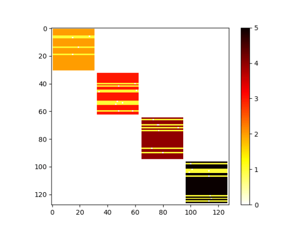
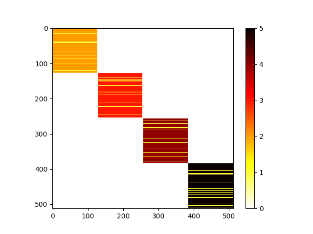
  • So here’s a pretty typical population. It’s 10% Explorer, 90% Exploiter. Exploit social influence radius is 0.2. These settings produce an orbiting flock. Between-group interaction is allowed, so This is a grid where the accumulated relationship of each agent to every other agent is shown. Red is closest, green is farthestcolorizedpositions You can see the different populations pretty well. One thing that isn’t that obvious is that exploiters are on average slightly closer to each other than to exploiters.
  • A more extreme example is where the Exploit influence distance is 10: colorizedpositions2 These tables show just relative position when compared to the origin.
  • Although I can’t figure out how to classify using this data, clustering works pretty well. This is Canopy (WEKA) on the top dataset above:
    === Run information ===
    
    Scheme: weka.clusterers.Canopy -N -1 -max-candidates 100 -periodic-pruning 10000 -min-density 2.0 -t2 -1.0 -t1 -1.25 -S 1
    Relation: ORIGIN_POSITION_DELTA
    Instances: 100
    Attributes: 102
    [list of attributes omitted]
    Test mode: Classes to clusters evaluation on training data
    
    === Clustering model (full training set) ===
    
    Canopy clustering
    =================
    
    Number of canopies (cluster centers) found: 2
    T2 radius: 3.137
    T1 radius: 3.922
    
    Cluster 0: 0.283631,0.443357,0.240249,0.280277,0.396611,0.258673,0.28608,0.27558,0.312295,0.215801,0.249255,0.25779,0.280719,0.273191,0.58818,0.258901,0.196191,0.240405,0.201927,0.273491,0.271862,0.266807,0.249377,0.269756,0.265874,0.252873,0.299417,0.244208,0.284257,0.253868,0.234348,0.213578,0.242031,0.248292,0.215259,0.236993,0.301843,0.245444,0.282464,0.290885,0.216585,0.375846,0.223493,0.278251,0.375965,0.764462,0.338657,0.280672,0.316447,0.261622,0.265026,0.436098,0.246442,0.246887,0.289306,0.470806,0.43541,0.209845,0.220971,0.21506,0.247576,0.249173,0.468053,0.28907,0.418987,0.293851,0.452858,0.267638,0.243671,0.248868,0.242674,0.371534,0.29843,0.221506,0.25575,0.242182,0.335877,0.28386,0.303986,0.235298,0.282083,0.427425,0.26635,0.251009,0.304134,0.281157,0.212644,0.367693,0.222213,0.247862,0.780248,0.894699,0.713413,0.865287,0.826024,0.868741,0.757008,0.807287,0.785141,0.756071,{88}
    Cluster 1: 0.919922,0.669721,0.908035,0.73578,0.591465,0.752733,0.774358,0.826861,0.84364,0.884803,0.939301,0.958981,0.629587,0.76459,0.545587,0.715267,0.853073,0.803545,0.851979,0.693952,0.954557,0.703606,0.897206,0.698297,0.926263,0.91898,0.733686,0.818759,0.763319,0.776199,0.843167,0.811708,0.903011,0.814435,0.804113,0.916336,0.639919,0.779399,0.663897,0.754696,0.77482,0.682512,0.832556,0.764008,0.703999,0.513612,0.693526,0.734279,0.723504,0.903016,0.777757,0.597915,0.86509,0.900357,0.724636,0.648915,0.577278,0.883327,0.828117,0.813873,0.860062,0.915821,0.684886,0.979451,0.556747,0.667678,0.556487,0.941671,0.898276,0.902846,0.686763,0.664381,0.709607,0.706246,0.890753,0.898794,0.588379,1.001214,0.625244,0.761188,0.828436,0.661864,0.759379,0.944355,0.728272,0.764909,0.761139,0.65028,0.845547,0.87213,0.586679,0.500194,0.498893,0.513267,0.493026,0.58192,0.620756,0.469854,0.540532,0.496272,{12}
    
    Time taken to build model (full training data) : 0.03 seconds
    
    === Model and evaluation on training set ===
    
    Clustered Instances
    
    0 88 ( 88%)
    1 12 ( 12%)
    
    Class attribute: AgentBias_
    Classes to Clusters:
    
    0 1 -- assigned to cluster
    0 10 | EXPLORER
    88 2 | EXPLOITER
    
    Cluster 0 -- EXPLOITER
    Cluster 1 -- EXPLORER
    
    Incorrectly clustered instances : 2.0 2 %
  • The next analyses is on the second dataset. They are essentially the same, even though the differences are more dramatic (the tight clusters are very tight
    === Run information ===
    
    Scheme:       weka.clusterers.Canopy -N -1 -max-candidates 100 -periodic-pruning 10000 -min-density 2.0 -t2 -1.0 -t1 -1.25 -S 1
    Relation:     ORIGIN_POSITION_DELTA
    Instances:    100
    Attributes:   102
                  [list of attributes omitted]
    Test mode:    Classes to clusters evaluation on training data
    
    === Clustering model (full training set) ===
    
    
    Canopy clustering
    =================
    
    Number of canopies (cluster centers) found: 2
    T2 radius: 3.438     
    T1 radius: 4.297     
    
    Cluster 0: 0.085848,0.050964,0.0513,0.053288,0.05439,0.054653,0.21758,0.057725,0.058775,0.050894,0.053768,0.130821,0.051098,0.050923,0.051115,0.050893,0.051012,0.051009,0.060649,0.051454,0.051089,0.051032,0.050894,0.053364,0.276684,0.051857,0.050984,0.050942,0.0509,0.050952,0.051025,0.056953,0.050914,0.050962,0.050903,0.052129,0.128196,0.051023,0.054222,0.274438,0.053978,0.050934,0.051124,0.054563,0.050995,0.074289,0.051077,0.05094,0.053644,0.050941,0.051343,0.050967,0.062704,0.052333,0.050936,0.051013,0.050922,0.051007,0.051038,0.050899,0.501239,0.051574,0.051005,0.050898,0.050944,0.204398,0.06076,0.050947,0.050904,0.408553,0.051263,0.0511,0.051574,0.069173,0.050997,0.162314,0.051353,0.096523,0.498648,0.339103,0.051125,0.050888,0.051002,0.051124,0.080711,0.05105,0.051024,0.050988,0.100492,0.132793,0.630178,0.882598,0.832132,0.86452,0.55151,0.729317,0.755526,0.513822,0.782104,0.768836,{92} 
    Cluster 1: 0.799117,0.793729,0.79643,0.7929,0.797843,0.797642,0.709935,0.78817,0.805937,0.794095,0.7972,0.76062,0.793743,0.79418,0.794846,0.794247,0.794677,0.793599,0.800359,0.794787,0.793849,0.793805,0.793613,0.784762,0.774656,0.79547,0.794308,0.793527,0.794406,0.793292,0.793513,0.800151,0.793775,0.793652,0.794123,0.793645,0.73331,0.794506,0.788542,0.710244,0.793332,0.793313,0.794184,0.801119,0.79448,0.802416,0.793669,0.7947,0.794813,0.794533,0.796484,0.794512,0.797614,0.794607,0.793716,0.793642,0.793548,0.794789,0.793551,0.793989,0.539133,0.79391,0.793443,0.793969,0.794472,0.715896,0.790956,0.794494,0.794293,0.678147,0.79434,0.793611,0.794221,0.802197,0.793753,0.759132,0.794164,0.798071,0.55929,0.698333,0.79444,0.79424,0.793585,0.793581,0.779958,0.79394,0.793567,0.794795,0.764686,0.754727,0.482214,0.518683,0.434538,0.501648,0.790616,0.4855,0.464554,0.691735,0.405411,0.496892,{8} 


    Time taken to build model (full training data) : 0.01 seconds
    
    === Model and evaluation on training set ===
    
    Clustered Instances
    
    0       88 ( 88%)
    1       12 ( 12%)
    
    
    Class attribute: AgentBias_
    Classes to Clusters:
    
      0  1  -- assigned to cluster
      0 10 | EXPLORER
     88  2 | EXPLOITER
    
    Cluster 0 -- EXPLOITER
    Cluster 1 -- EXPLORER
    
    Incorrectly clustered instances :	2.0	  2      %
  • Online clustering, fear and uncertainty in Egypt’s transition (Published today). Wow. Downloaded

11:00 – 6:00 BRC

  • Spent the rest of the day working on the CHIMERA paper with Aaron

Phil 2.17.17

7:00 – 8:00 research

  • I think I want to navigate the information space of Trump’s tweets
  • Still working on how to classify an agent. After struggling a bit, I can classify very well if I eliminate extraneous infor from mean angle stats, leaving only bias and variance

8:30 – 10:30, 4:00 – 5:00

  • Working on creating, extracting and classifying cluster membership from flocks.
  • Had to leave early to help Barbara with Buck
  • Discussed exec summary with Aaron. Will write on Monday

Phil 2.16.17

7:00 – 8:00 Research

  • Had a great time NOT DOING ANY THINKING yesterday
  • Rechecking the velocity comparison matrix. It’s correct. Looking at multiplying or adding relative position vs relative velocity
  • Sent a few charts to Don to see if he can make anything pretty
  • Uploaded new version

8:30 – 5:00 BRC

Phil 2.14.17

7:00 – 8:00 Research

  • Based on the charts from yesterday, I think I’m going to build two matrices to point WEKA at. Essentially, theses matrices will be filled with meta-cluster information
    • Average distance from agent to agent. Tightly clustered agents should have low average distances. DBSCAN should also work on this, as well as bootstrapping. That should cover this case: exploit_vs_exploit
    • Average velocity from agent to agent. I’m not sure what I’ll get from this, but in looking at the explore-explore case and the explore-exploit case, it strikes me that there may be some difference that is meaningful. And in the exploit-exploit case, the velocities should be near zero explore_vs_exploit Explore-exploitexplore_vs_explore Explore-explore
    • Start with Excel, and then add an ARFF
      • Got most of the methods built. Might finish this morning at work.
      • Indeed, you can get a lot done when you’re sitting in on a Skype meeting and they’re not talking about your part…
      • Ok, so I’ve added comparison matrices as Excel and ARFF output. In this case WEKA does better charting, so here goes. The first chart is exploit-exploit. Note that the majority of points are at 0,0: explit-exploit-deltas Next, an explore-exploit. In this case, there’s a cluster on the left side of the chart: exploit-explore-deltasLast, is the explore-explore chart, which has a cluster towards the middle: explore-explore-deltas
      • This data also seems to be good to train a NaiveBayes Classifier. Here’s the result of an initial run:
        === Stratified cross-validation ===
        === Summary ===
        
        Correctly Classified Instances          97               97      %
        Incorrectly Classified Instances         3                3      %
        Kappa statistic                          0.94  
        Mean absolute error                      0.03  
        Root mean squared error                  0.1732
        Relative absolute error                  6      %
        Root relative squared error             34.6337 %
        Total Number of Instances              100     
        
        === Detailed Accuracy By Class ===
        
                         TP Rate  FP Rate  Precision  Recall   F-Measure  MCC      ROC Area  PRC Area  Class
                         1.000    0.059    0.942      1.000    0.970      0.942    0.971     0.942     EXPLORER
                         0.941    0.000    1.000      0.941    0.970      0.942    1.000     1.000     EXPLOITER
        Weighted Avg.    0.970    0.029    0.972      0.970    0.970      0.942    0.986     0.972     
        
        === Confusion Matrix ===
        
          a  b   -- classified as
         49  0 |  a = EXPLORER
          3 48 |  b = EXPLOITER
      • Velocity also works, the plots aren’t as crisp, but the classifier accuracy is about the same: exploit-exploit-velocity Exploit-Exploit exploit-explore-velocity Explore-Exploit explore-explore-velocity Explore-Explore
      • Again, classification looks good:
        === Stratified cross-validation ===
        === Summary ===
        
        Correctly Classified Instances          99               99      %
        Incorrectly Classified Instances         1                1      %
        Kappa statistic                          0.98  
        Mean absolute error                      0.01  
        Root mean squared error                  0.1   
        Relative absolute error                  2      %
        Root relative squared error             19.9957 %
        Total Number of Instances              100     
        
        === Detailed Accuracy By Class ===
        
                         TP Rate  FP Rate  Precision  Recall   F-Measure  MCC      ROC Area  PRC Area  Class
                         1.000    0.020    0.980      1.000    0.990      0.980    1.000     1.000     EXPLORER
                         0.980    0.000    1.000      0.980    0.990      0.980    1.000     1.000     EXPLOITER
        Weighted Avg.    0.990    0.010    0.990      0.990    0.990      0.980    1.000     1.000     
        
        === Confusion Matrix ===
        
          a  b   -- classified as
         49  0 |  a = EXPLORER
          1 50 |  b = EXPLOITER
    • Uploaded new version of the tool to philfeldman.com/GroupPolarization/GroupPloarizationModel.jar

8:30 – 3:30. BRC

  • Either start on the ResearchBrowser or continue with meta-clustering.
  • Grooming and sprint planning today – done! And good progress while hanging out on the phone.

Phil 2.13.17

7:00 – 8:00, 3:00 – 5:30 Research

  • Getting the toArff methods working with the WEKA date format: The default format string accepts the ISO-8601 combined date and time format: yyyy-MM-dd'T'HH:mm:ss
  • Going to go with Milliseconds format, and then set the ARFF to default to 1 sec increments. Nope, that didn’t work. Going with the default fromat and incrementing by seconds.
  • Fika
  • Meeting with Wayne. Basically catching up, but I also got to show him the sim. And for a numerical model of community behavior based on sociophysics, we got into a very involved conversation. Visualization helps tell stories.

8:30 – 2:30 BRC

  • Testing periodicity and time series classifiers
  • I can forecast in a bunch of different ways, but I can’t seem to classify. There are several filters, but no real explanation
  • Redoing some simulations, to see the best way of checking for Explorer/exploiter behavior. Here are some screenshots:
  • Explore-Explore explore_vs_explore
  • Explore-Exploit explore_vs_exploit
  • Exploit-Exploit exploit_vs_exploit