
7:00 – 4:30 ASRC GOES
- FractalNet: Ultra-Deep Neural Networks without Residuals
- We introduce a design strategy for neural network macro-architecture based on self-similarity. Repeated application of a simple expansion rule generates deep networks whose structural layouts are precisely truncated fractals. These networks contain interacting subpaths of different lengths, but do not include any pass-through or residual connections; every internal signal is transformed by a filter and nonlinearity before being seen by subsequent layers. In experiments, fractal networks match the excellent performance of standard residual networks on both CIFAR and ImageNet classification tasks, thereby demonstrating that residual representations may not be fundamental to the success of extremely deep convolutional neural networks. Rather, the key may be the ability to transition, during training, from effectively shallow to deep. We note similarities with student-teacher behavior and develop drop-path, a natural extension of dropout, to regularize co-adaptation of subpaths in fractal architectures. Such regularization allows extraction of high-performance fixed-depth subnetworks. Additionally, fractal networks exhibit an anytime property: shallow subnetworks provide a quick answer, while deeper subnetworks, with higher latency, provide a more accurate answer.
- Structural diversity in social contagion
- The concept of contagion has steadily expanded from its original grounding in epidemic disease to describe a vast array of processes that spread across networks, notably social phenomena such as fads, political opinions, the adoption of new technologies, and financial decisions. Traditional models of social contagion have been based on physical analogies with biological contagion, in which the probability that an individual is affected by the contagion grows monotonically with the size of his or her “contact neighborhood”—the number of affected individuals with whom he or she is in contact. Whereas this contact neighborhood hypothesis has formed the underpinning of essentially all current models, it has been challenging to evaluate it due to the difficulty in obtaining detailed data on individual network neighborhoods during the course of a large-scale contagion process. Here we study this question by analyzing the growth of Facebook, a rare example of a social process with genuinely global adoption. We find that the probability of contagion is tightly controlled by the number of connected components in an individual’s contact neighborhood, rather than by the actual size of the neighborhood. Surprisingly, once this “structural diversity” is controlled for, the size of the contact neighborhood is in fact generally a negative predictor of contagion. More broadly, our analysis shows how data at the size and resolution of the Facebook network make possible the identification of subtle structural signals that go undetected at smaller scales yet hold pivotal predictive roles for the outcomes of social processes.
- Add this to the discussion section – done
- Dissertation
- Started on the theory section, then realized the background section didn’t set it up well. So worked on the background instead. I put in a good deal on how individuals and groups interact with the environment differently and how social interaction amplifies individual contribution through networking.
- Quick meetings with Don and Aaron
- Time prediction (sequence to sequence) with Keras perceptrons


- This was surprisingly straightforward
- There was some initial trickiness in getting the IDE to work with the TF2.0 RC0 package:
import tensorflow as tf
from tensorflow import keras
from tensorflow_core.python.keras import layers
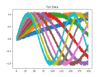
The first coding step was to generate the data. In this case I’m building a numpy matrix that has ten variations on math.sin(), using our timeseriesML utils code. There is a loop that sets up the code to create a new frequency, which is sent off to get back a pandas Dataframe that in this case has 10 sequence rows with 100 samples. First, we set the global sequence_length:
sequence_length = 100
then we create the function that will build and concatenate our numpy matrices:
def generate_train_test(num_functions, rows_per_function, noise=0.1) -> (np.ndarray, np.ndarray, np.ndarray):
    ff = FF.float_functions(rows_per_function, 2*sequence_length)
    npa = None
    for i in range(num_functions):
        mathstr = "math.sin(xx*{})".format(0.005*(i+1))
        #mathstr = "math.sin(xx)"
        df2 = ff.generateDataFrame(mathstr, noise=0.1)
        npa2 = df2.to_numpy()
        if npa is None:
            npa = npa2
        else:
            ta = np.append(npa, npa2, axis=0)
            npa = ta

    split = np.hsplit(npa, 2)
    return npa, split[0], split[1]
Now, we build the model. We’re using keras from the TF 2.0 RC0 build, so things look slightly different:
model = tf.keras.Sequential()
# Adds a densely-connected layer with 64 units to the model:
model.add(layers.Dense(sequence_length, activation='relu', input_shape=(sequence_length,)))
# Add another:
model.add(layers.Dense(200, activation='relu'))
# Add a softmax layer with 10 output units:
model.add(layers.Dense(sequence_length))

loss_func = tf.keras.losses.MeanSquaredError()
opt_func = tf.keras.optimizers.Adam(0.01)
model.compile(optimizer= opt_func,
              loss=loss_func,
              metrics=['accuracy'])
We can now fit the model to the generated data:
full_mat, train_mat, test_mat = generate_train_test(10, 10)

model.fit(train_mat, test_mat, epochs=10, batch_size=2)
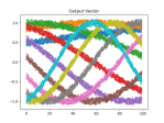
There is noise in the data, so the accuracy is not bang on, but the loss is nice. We can see this better in the plots above, which were created using this function:
def plot_mats(mat:np.ndarray, cluster_size:int, title:str, fig_num:int):
    plt.figure(fig_num)

    i = 0
    for row in mat:
        cstr = "C{}".format(int(i/cluster_size))
        plt.plot(row, color=cstr)
        i += 1

    plt.title(title)
Which is called just before the program completes:
if show_plots: plot_mats(full_mat, 10, "Full Data", 1) plot_mats(train_mat, 10, "Input Vector", 2) plot_mats(test_mat, 10, "Output Vector", 3) plot_mats(predict_mat, 10, "Predict", 4) plt.show() - That’s it! Full listing below:
- There was some initial trickiness in getting the IDE to work with the TF2.0 RC0 package:
import tensorflow as tf
from tensorflow import keras
from tensorflow_core.python.keras import layers
import numpy as np
import pandas as pd
import matplotlib.pyplot as plt
import timeseriesML.generators.float_functions as FF


sequence_length = 100

def generate_train_test(num_functions, rows_per_function, noise=0.1) -> (np.ndarray, np.ndarray, np.ndarray):
    ff = FF.float_functions(rows_per_function, 2*sequence_length)
    npa = None
    for i in range(num_functions):
        mathstr = "math.sin(xx*{})".format(0.005*(i+1))
        #mathstr = "math.sin(xx)"
        df2 = ff.generateDataFrame(mathstr, noise=0.1)
        npa2 = df2.to_numpy()
        if npa is None:
            npa = npa2
        else:
            ta = np.append(npa, npa2, axis=0)
            npa = ta

    split = np.hsplit(npa, 2)
    return npa, split[0], split[1]

def plot_mats(mat:np.ndarray, cluster_size:int, title:str, fig_num:int):
    plt.figure(fig_num)

    i = 0
    for row in mat:
        cstr = "C{}".format(int(i/cluster_size))
        plt.plot(row, color=cstr)
        i += 1

    plt.title(title)

model = tf.keras.Sequential()
# Adds a densely-connected layer with 64 units to the model:
model.add(layers.Dense(sequence_length, activation='relu', input_shape=(sequence_length,)))
# Add another:
model.add(layers.Dense(200, activation='relu'))
# Add a softmax layer with 10 output units:
model.add(layers.Dense(sequence_length))

loss_func = tf.keras.losses.MeanSquaredError()
opt_func = tf.keras.optimizers.Adam(0.01)
model.compile(optimizer= opt_func,
              loss=loss_func,
              metrics=['accuracy'])

full_mat, train_mat, test_mat = generate_train_test(10, 10)

model.fit(train_mat, test_mat, epochs=10, batch_size=2)
model.evaluate(train_mat, test_mat)

# test against freshly generated data
full_mat, train_mat, test_mat = generate_train_test(10, 10)
predict_mat = model.predict(train_mat)

show_plots = True
if show_plots:
    plot_mats(full_mat, 10, "Full Data", 1)
    plot_mats(train_mat, 10, "Input Vector", 2)
    plot_mats(test_mat, 10, "Output Vector", 3)
    plot_mats(predict_mat, 10, "Predict", 4)
    plt.show()
