7:30 – 4:00 BRC

• Bike to work day. Must’ve missed Mike
• Tried to program the phone, but no pause for teleconf.
• Still no Jira.
• Working on documentation
• Clustering meeting with Shawn, Aaron and Ellis?
• PubMed search for ICD code Clustering. Not that much???

Research

• Locally noisy autonomous agents improve global human coordination in network experiments

7:00 – 8:00 Research

• Updated CV.
• We tracked the Trump scandals on right-wing news sites. Here’s how they covered it. This is an article by Vox that might be good to look at a belief/information flow over time.
• A Tale of Two Moralities, Part One: Regional Inequality and Moral Polarization
• Working on HCIC poster
• Social identity theory? No – Self-categorization theory
  • Polarized Norms and Social Frames of Reference: A Test of the Self-Categorization Theory of Group Polarization

8:30 – 3:45 BRC

• Still getting pushback on workstation. Ordered?
• Still no Jira connectivity
• Got a phone!
• Cleaning up and documenting code

7:00 – 8:00 Research

• Media Manipulation and Disinformation Online (Alice Marwick and Rebecca Lewis)
• Call for Papers: Special Issue on Computational Propaganda and Political Big Data
• Authoritarianism and Post-truth Politics
• HCIC poster (June 2)
• PhD Review (May 26) – done!
  • Update CV!

8:30 – 4:30 BRC

• Meetings. All. Day. Long.
• Finished transferring Aaron’s ppt to LaTex. Looks pretty good, and an excellent first draft
  • We need to publish as a baseline to reference for our methods and choices. If it makes it through the review process, then we can point to it when we’re called out like in this morning’s review

7:00 – 8:00 Research

• Never made it to Fika yesterday. Worked a solid 13.5 hours. Artificial deadlines are pretty dumb.
• Continuing with registration paperwork and other loose ends
  • HCIC travel (May 19), poster (June 2) – Attempting to register. Account created
    • Registered!
    • Travel email sent. Sat June 24 – Sat Jul 1
  • PhD Review (May 26) – started. Sure hope It incrementally saves…
    • Nope – starting over, offline. Making progress…

9:00 – 5:00 BRC

• Sprint review. Went well, I think
• Working on turning the PPT into a document

Well, the weekend ended on a sad, down note. Having problems getting motivated.

7:00 – 8:00 Research

• Filled out CI 2017 form
• Started HCIC registration
• Started PhD review

8:30 – 8:00PM BRC

• Run clustering on t-SNE again with Bob’s settings. It’s…. OK. We think that MDS and LLE are better for now, but there are almost certainly hyper parameter tweaking that we can do.
• Here’s n example of actual data with lots of error between runs: but by adjusting the hyperparameter ‘neighbors’ from 5 (above) to 10 (below), we get a completely different result: Here, you can see that no cluster shared its nodes with any other cluster. That’s what we want. Stable, but with good granularity.
• We can play some games on the clustering by seeing what happens when we remove some columns from our data. Here’s the above data with gender included and excluded: It’s possible to see that several items that were in cluster (0) distribute out when gender don’t override associated clusters.
• Had a weird issue where LLE clustering on our test data that worked with neighbors = 10, now needs neighbors > 12 to work. Not sure why that’s happening.
• Need to write up a report generator that does the following:  For each cluster in the set that we are comparing:
  

  size
  stable/total
  list of stable

Tasks:

• Collective Intelligence details (May 18) – Done
• HCIC travel (May 19), poster (June 2) – Attempting to register. Account created
• PhD Review (May 26) – started. Sure hope It incrementally saves…
• CHIIR 2018
  • 1 October 2017 *- Full papers and Perspectives papers due
  • 22 October 2017* – Short papers, Demos, Workshops and Tutorials proposals due
  • 1 November 2017* – Doctoral Consortium applications due
  • 15 December 2017* – Notification of acceptance

7:00 – 8:00 Research

• I searched for better Electome images (unannotated) and found a few. They are on the previous post. I’ll seriously start to work on the poster this weekend.
• Cleaned up some code, and made the writing of an image file optional. Still figuring out the best way to do helper classes in Python
• Starting to learn the analytic capabilities of Networkx, which is its core as I understand. Going to start to characterize the networks and compare against stored sets (like the Karate Club) that is in the library
• List of algorithms

8:30 – 4:30 BRC

• Working on cluster member sequence visualization.
  • Needed to make unclustered user configurable
  • Needed to make timeline sequence, where OPEN and CLOSED states are enabled, user configurable
• Results! LLE looks to be the best by far:

  

  

  

  

  

  
  

7:00 – 8:00, 4:00-7:00 Research

• Guest lecture for CSCW class! Notes!
  • And it went well. Fun, actually.
• Working on making the line width based on the time spent in the cluster, the cluster size a function of its lifespan, and the agent size, a function of time spent in a cluster
  • While working on the last part, I realized that I was including ‘unclustered’ (-1) as a cluster. This made all the agents the same size, and also messed up the cluster collating, since unclustered can be the majority in some circumstances. Fixing this made everything much better: so now I need to rerun all the variations. Done! Rough boaster poster:
• Found better Electome images. More project info here and here: 

9:00 – 3:00 BRC

• Finished temporal coherence. Now we can compare across multiple cluster attempts. Tomorrow I’ll set up the cluster_optomizer to make multiple runs and produce an Excel file containing columns of cluster attempts

7:00 – 8:00

• Systematic exploration of unsupervised methods for mapping behavior
• Thinking about the stories I can tell with the GP sim.
  • Start together with same settings.
  • Disconnect
  • Slide exploit to max
• Need to download blog entries
• Working on graphing. Success!!!!! Now I need to discriminate agents from clusters, and exploit from explore. But this shows polarized vs. diverse clustering. I’m pretty sure I can get all kinds of statistics out of this too!
• Better version. Ran all the permutations:
• explore_1.6_exploit_3.2_ran 04_14_17-08_38_48. Green are clusters, Red are Exploit, Blue are Explore
• Need to make the line width based on the time spent in the cluster, and the cluster size a function of its lifespan

9:00 – 5:00 BRC

• Working on showing where the data broke. Looks like Talend
• For future referrence, How to turn a dict of rows into a DataFrame and then how to access all the parts:

  import pandas as pd
  
  d1 = {'one':1.1, 'two':2.1, 'three':3.1}
  d2 = {'one':1.2, 'three':3.2}
  d3 = {'one':1.3, 'two':2.3, 'three':3.3}
  rows = {'row1':d1, 'row2':d2}
  rows['row3'] = d3
  df = pd.DataFrame(rows)
  df = df.transpose()
  print(df)
  
  for index, row in df.iterrows():
      print(index)
      for key, val in row.iteritems():
          print("{0}:{1}".format(key, val))

• Helped Aaron with the writeups
• And it turns out that all the work I did “could be done in an hour”. So back to clustering and AI work. If there is a problem with the data, I know that it works with the test data. Others can figure out where the problem is, since they can handle it so quickly.

7:00 – 8:00 Research

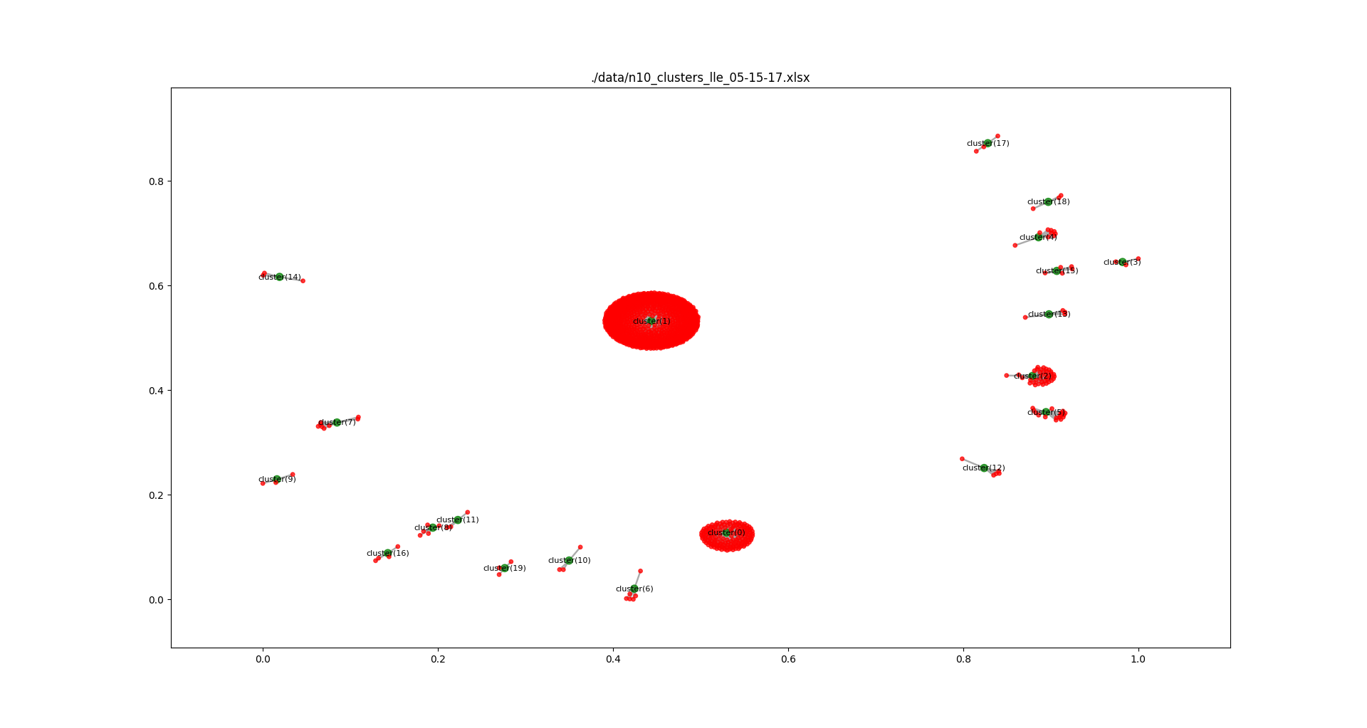
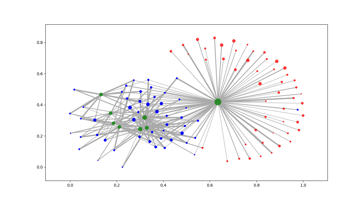
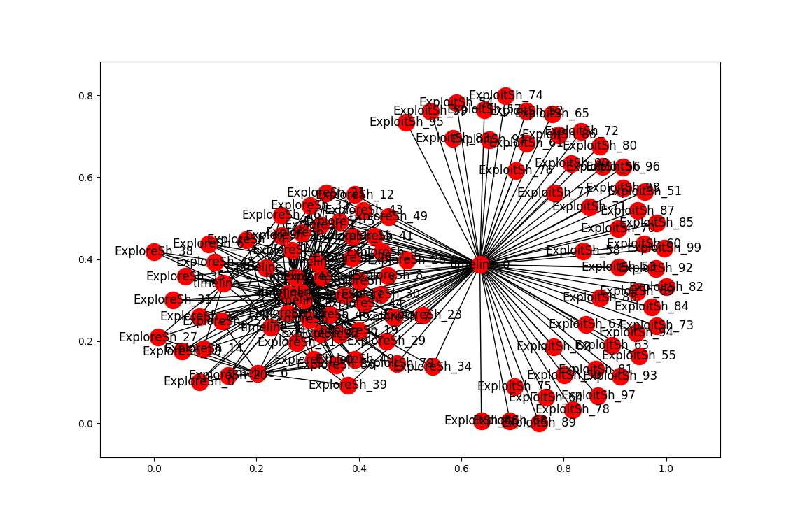
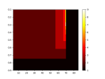
• More clustering. Here’s the list of agents by clusters. An OPEN state means that the simulation finished with agents in the cluster. Num_entries is: the lifetime of the cluster. For these runs, the max is 200. Id is the ‘name’ of the cluster. Tomorrow, I’ll try to get this drawn using networkx.

  timeline[0]:
  Id = cluster_0
  State = ClusterState.OPEN
  Num entries = 200
  {'ExploitSh_52', 'ExploreSh_43', 'ExploitSh_56', 'ExploreSh_2', 'ExploreSh_5', 'ExploitSh_73', 'ExploitSh_95', 'ExploreSh_19', 'ExploreSh_4', 'ExploitSh_87', 'ExploitSh_76', 'ExploreSh_3', 'ExploitSh_93', 'ExploreSh_32', 'ExploreSh_41', 'ExploreSh_17', 'ExploitSh_88', 'ExploitSh_77', 'ExploreSh_39', 'ExploitSh_85', 'ExploreSh_40', 'ExploitSh_64', 'ExploreSh_34', 'ExploreSh_22', 'ExploitSh_99', 'ExploreSh_1', 'ExploitSh_97', 'ExploitSh_69', 'ExploreSh_29', 'ExploitSh_58', 'ExploitSh_62', 'ExploreSh_23', 'ExploreSh_36', 'ExploreSh_11', 'ExploitSh_80', 'ExploitSh_82', 'ExploreSh_21', 'ExploitSh_75', 'ExploitSh_72', 'ExploitSh_89', 'ExploitSh_86', 'ExploreSh_37', 'ExploitSh_84', 'ExploitSh_81', 'ExploreSh_15', 'ExploitSh_51', 'ExploreSh_44', 'ExploitSh_83', 'ExploitSh_94', 'ExploreSh_16', 'ExploitSh_53', 'ExploitSh_67', 'ExploitSh_74', 'ExploreSh_45', 'ExploreSh_26', 'ExploreSh_12', 'ExploreSh_13', 'ExploitSh_92', 'ExploreSh_9', 'ExploreSh_28', 'ExploitSh_50', 'ExploreSh_8', 'ExploreSh_30', 'ExploreSh_49', 'ExploitSh_59', 'ExploitSh_57', 'ExploreSh_42', 'ExploitSh_65', 'ExploitSh_54', 'ExploitSh_61', 'ExploitSh_66', 'ExploitSh_55', 'ExploitSh_78', 'ExploitSh_68', 'ExploitSh_79', 'ExploitSh_91', 'ExploitSh_71', 'ExploreSh_7', 'ExploitSh_98', 'ExploitSh_60', 'ExploitSh_70', 'ExploreSh_10', 'ExploitSh_90', 'ExploreSh_46', 'ExploitSh_96', 'ExploreSh_47', 'ExploitSh_63'}
  
  timeline[1]:
  Id = cluster_1
  State = ClusterState.OPEN
  Num entries = 200
  {'ExploreSh_25', 'ExploreSh_6', 'ExploreSh_38', 'ExploreSh_43', 'ExploreSh_49', 'ExploreSh_1', 'ExploreSh_2', 'ExploreSh_20', 'ExploreSh_33', 'ExploreSh_48', 'ExploreSh_5', 'ExploreSh_29', 'ExploreSh_15', 'ExploreSh_42', 'ExploreSh_24', 'ExploreSh_19', 'ExploreSh_4', 'ExploreSh_44', 'ExploreSh_16', 'ExploreSh_23', 'ExploreSh_36', 'ExploreSh_11', 'ExploreSh_3', 'ExploreSh_27', 'ExploreSh_35', 'ExploreSh_32', 'ExploreSh_17', 'ExploreSh_26', 'ExploreSh_21', 'ExploreSh_12', 'ExploreSh_18', 'ExploreSh_45', 'ExploreSh_41', 'ExploitSh_79', 'ExploreSh_13', 'ExploreSh_0', 'ExploreSh_39', 'ExploreSh_7', 'ExploreSh_9', 'ExploreSh_28', 'ExploreSh_40', 'ExploreSh_31', 'ExploreSh_10', 'ExploreSh_46', 'ExploreSh_37', 'ExploreSh_14', 'ExploreSh_47', 'ExploreSh_8', 'ExploreSh_30', 'ExploreSh_34', 'ExploreSh_22'}
  
  timeline[2]:
  Id = cluster_2
  State = ClusterState.CLOSED
  Num entries = 56
  {'ExploreSh_25', 'ExploreSh_1', 'ExploreSh_33', 'ExploreSh_29', 'ExploreSh_5', 'ExploreSh_48', 'ExploreSh_15', 'ExploreSh_19', 'ExploreSh_36', 'ExploreSh_3', 'ExploreSh_11', 'ExploreSh_35', 'ExploreSh_45', 'ExploreSh_17', 'ExploreSh_26', 'ExploreSh_41', 'ExploitSh_79', 'ExploreSh_13', 'ExploreSh_9', 'ExploreSh_40', 'ExploreSh_31', 'ExploreSh_37', 'ExploreSh_47', 'ExploreSh_30', 'ExploreSh_22'}
  
  timeline[3]:
  Id = cluster_3
  State = ClusterState.CLOSED
  Num entries = 16
  {'ExploreSh_25', 'ExploreSh_6', 'ExploreSh_43', 'ExploreSh_2', 'ExploreSh_48', 'ExploreSh_5', 'ExploreSh_15', 'ExploreSh_42', 'ExploreSh_24', 'ExploreSh_4', 'ExploreSh_44', 'ExploreSh_3', 'ExploreSh_26', 'ExploreSh_17', 'ExploreSh_41', 'ExploreSh_21', 'ExploreSh_32', 'ExploreSh_13', 'ExploreSh_9', 'ExploreSh_7', 'ExploreSh_28', 'ExploreSh_37', 'ExploreSh_8', 'ExploreSh_30', 'ExploreSh_49', 'ExploreSh_22'}
  
  timeline[4]:
  Id = cluster_4
  State = ClusterState.CLOSED
  Num entries = 30
  {'ExploreSh_6', 'ExploreSh_1', 'ExploreSh_2', 'ExploreSh_20', 'ExploreSh_33', 'ExploreSh_48', 'ExploreSh_15', 'ExploreSh_24', 'ExploreSh_4', 'ExploreSh_16', 'ExploreSh_23', 'ExploreSh_3', 'ExploreSh_11', 'ExploreSh_26', 'ExploreSh_41', 'ExploreSh_17', 'ExploreSh_32', 'ExploreSh_18', 'ExploreSh_13', 'ExploreSh_9', 'ExploreSh_46', 'ExploreSh_37', 'ExploreSh_8', 'ExploreSh_30', 'ExploreSh_49', 'ExploreSh_22'}
  
  timeline[5]:
  Id = cluster_5
  State = ClusterState.CLOSED
  Num entries = 28
  {'ExploreSh_25', 'ExploreSh_43', 'ExploreSh_2', 'ExploreSh_48', 'ExploreSh_29', 'ExploreSh_42', 'ExploreSh_24', 'ExploreSh_4', 'ExploreSh_44', 'ExploreSh_36', 'ExploreSh_35', 'ExploreSh_45', 'ExploreSh_17', 'ExploreSh_26', 'ExploreSh_12', 'ExploreSh_0', 'ExploreSh_28', 'ExploreSh_40', 'ExploreSh_31', 'ExploreSh_46', 'ExploreSh_37', 'ExploreSh_14', 'ExploreSh_47', 'ExploreSh_8', 'ExploreSh_30', 'ExploreSh_22'}
  
  timeline[6]:
  Id = cluster_6
  State = ClusterState.CLOSED
  Num entries = 10
  {'ExploreSh_40', 'ExploreSh_25', 'ExploreSh_18', 'ExploreSh_27', 'ExploreSh_10', 'ExploreSh_13', 'ExploreSh_20', 'ExploreSh_0', 'ExploreSh_37', 'ExploreSh_14', 'ExploreSh_36', 'ExploreSh_11', 'ExploreSh_39', 'ExploreSh_42', 'ExploreSh_22'}
  
  timeline[7]:
  Id = cluster_7
  State = ClusterState.CLOSED
  Num entries = 9
  {'ExploreSh_38', 'ExploreSh_2', 'ExploreSh_4', 'ExploreSh_46', 'ExploreSh_16', 'ExploreSh_33', 'ExploreSh_47', 'ExploreSh_14', 'ExploreSh_11', 'ExploreSh_27', 'ExploreSh_35', 'ExploreSh_45'}
  
  timeline[8]:
  Id = cluster_8
  State = ClusterState.CLOSED
  Num entries = 25
  {'ExploreSh_21', 'ExploreSh_38', 'ExploreSh_19', 'ExploreSh_2', 'ExploreSh_13', 'ExploreSh_44', 'ExploreSh_1', 'ExploreSh_10', 'ExploreSh_16', 'ExploreSh_47', 'ExploreSh_5', 'ExploreSh_48', 'ExploreSh_42', 'ExploreSh_35', 'ExploreSh_22', 'ExploreSh_32'}
  
  timeline[9]:
  Id = cluster_9
  State = ClusterState.OPEN
  Num entries = 16
  {'ExploreSh_17', 'ExploreSh_6', 'ExploreSh_24', 'ExploreSh_19', 'ExploreSh_10', 'ExploreSh_20', 'ExploreSh_46', 'ExploreSh_33', 'ExploreSh_14', 'ExploreSh_3', 'ExploreSh_39', 'ExploreSh_7', 'ExploreSh_45'}

• Network Dynamics and Simulation Science Laboratory – need to go through publications and venues for these folks
• Dynamic Spirals Put to Test: An Agent-Based Model of Reinforcing Spirals Between Selective Exposure, Interpersonal Networks, and Attitude Polarization
  • Within the context of partisan selective exposure and attitude polarization, this study investigates a mutually reinforcing spiral model, aiming to clarify mechanisms and boundary conditions that affect spiral processes—interpersonal agreement and disagreement, and the ebb and flow of message receptions. Utilizing agent-based modeling (ABM) simulations, the study formally models endogenous dynamics of cumulative processes and its reciprocal effect of media choice behavior over extended periods of time. Our results suggest that interpersonal discussion networks, in conjunction with election contexts, condition the reciprocal effect of selective media exposure and its attitudinal consequences. Methodologically, results also highlight the analytical utility of computational social science approaches in overcoming the limitations of typical experimental and observations studies.

8:30 – 5:30 BRC

• Logical Graphs: Control Flow in TensorFlow – Sam Abrahams (slides)
• Went digging through the input data. It is *not* the same. Generated lots of data
• When checking, we can tell that the data in the database is the same as it was in January
• Now looking to see if the data on CI is good

7:00 – 8:00 Research

• INTEL-SA-00075 vulnerability! Download and run Intel-SA-00075-GUI!
• A good weekend off. Big, cathartic 88 mile ride on Sunday, and the Kinetic Sculpture race on Saturday
• Working on the cluster visualization. Updating Intellij at home first
  • installed networkx
  • networkx_tutorial (Code from this post)is working
  • installed xlrd
  • membership_history_builder is working
  • Working on printing out the memberships, then I’ll start diagramming
• Thinking about how to start Thursday. I think I’ll try reading in blogs to LMN and show differences between students. then bring up flocking, then go into the material

8:30 – 4:00 BRC

• Analyzing data
• Showed Aaron the results on the generated and actual data. He’s pretty happy
  • Column mismatches between January and current data
  • Present in Jan data, but not in May:
    • First Excel crash of the day
    • Got the column difference working. It’s pretty sweet, actually:

      df1_cols = set(df1.columns.values)
      df2_cols = set(df2.columns.values)
      
      diff_cols = df2_cols ^ df1_cols

      That’s it.

    • Generated a report on different columns. Tomorrow I need to build a reduced DataFrame that has only the common columns, sort both on column names and then iterate to find the level of similarity.
  • Something’s wrong with?

    calc_naive_fitness_landscape()

Research 7:00 – 8:00

• Some interesting books:
  • Facing the Planetary: Entangled Humanism and the Politics of Swarming: Connolly focuses on the gap between those regions creating the most climate change and those suffering most from it. He addresses the creative potential of a “politics of swarming” by which people in different regions and social positions coalesce to reshape dominant priorities.
  • Medialogies: Reading Reality in the Age of Inflationary Media:  The book invites us to reconsider the way reality is constructed, and how truth, sovereignty, agency, and authority are understood from the everyday, philosophical, and political points of view.
  • At the Crossroads: Lessons and Challenges in Computational Social Science With tools borrowed from Statistical Physics and Complexity, this new area of study have already made important contributions, which in turn have fostered the development of novel theoretical foundations in Social Science and Economics, via mathematical approaches, agent-based modelling and numerical simulations. [free download!]
• Finished Online clustering, fear and uncertainty in Egypt’s transition. Notes are here
• The compass within Head direction cells have been hypothesized to form representations of an animal’s spatial orientation through internal network interactions. New data from mice show the predicted signatures of these internal dynamics. 
  • I wonder if these neurons are fired when information orientation changes?

8:30 – 3:00 BRC

• Giving up on graph-tool since I can’t get it installed. Trying plotly next. Nope. Expensive and too html-y. Networkx for the win? Starting the tutorial
  • Well this is really cool: You might notice that nodes and edges are not specified as NetworkX objects. This leaves you free to use meaningful items as nodes and edges. The most common choices are numbers or strings, but a node can be any hashable object (except None), and an edge can be associated with any object x using G.add_edge(n1,n2,object=x).
  • Very nice. And with this, I am *done* for the week:

    import networkx as nx
    import matplotlib.pyplot as plt
    
    #  Create the graph
    G=nx.Graph(name="test", creator="Phil")
    
    #  Create the nodes. Can be anything but None
    G.add_node("foo")
    G.add_node("bar")
    G.add_node("baz")
    
    #  Link edges to nodes
    G.add_edge("foo", "bar")
    G.add_edge("foo", "baz")
    G.add_edge("bar", "baz")
    
    #  Draw
    #  Set the positions using a layout
    pos=nx.circular_layout(G) # positions for all nodes
    
    #  Draw the nodes, setting size transparancy and color explicitly
    nx.draw_networkx_nodes(G, pos,
                    nodelist=["foo", "bar"],
                    node_color='g',
                    node_size=300,
                    alpha=0.5)
    nx.draw_networkx_nodes(G, pos,
                    nodelist=["baz"],
                    node_color='b',
                    node_size=600,
                    alpha=0.5)
    
    #  Draw edges and labels using defaults
    nx.draw_networkx_edges(G,pos)
    nx.draw_networkx_labels(G,pos)
    
    #  Render to pyplot
    plt.show()
    
    print("G.graph = {0}".format(G.graph))
    print("G.number_of_nodes() = {0}".format(G.number_of_nodes()))
    print("G.number_of_edges() = {0}".format(G.number_of_edges()))
    print("G.adjacency_list() = {0}".format(G.adjacency_list()))

  • 
• Short term goals
  • Show that it works in reasonable ways on our well characterized test data
  • See how much clustering changes from run to run
  • Compare differences between manifold learning techniques
  • Examine how it maps to the individual user data

Star wars day

7:00 – 8:00, 4:00 – 6:00 Research

• Continuing Online clustering, fear and uncertainty in Egypt’s transition. Notes are here
• Meeting with Wayne
  • Current trajectory is good
    • HCIC poster with clusters
    • What to do July+? Build ResearchBrowser. Anything else?
    • Also, try to put together a summary in the blog before each meeting
  • Add Wayne as coauthor if we get through the next gate
  • Got to talk about the future of work. My perspective is that machines will be able to meet all needs essentially for free, so we need to build an economy on a human value-add, like the Bugatti Veyron. The goal is to support the creation of items/experiences with a human value-add and an economy built around that.

8:30 – 3:30

• Fixing all of the broken code on CI
• Migrated all the machine-learning python code so everything matches
• changed the algorithm from subdivision to naive
• Working on CI

  t-SNE: 15 sec
  New best cluster: EPS = 0.1, Cluster size = 3.0
  clusters = 17
  Total  = 1179
  clustered = 1042
  unclustered = 137
  
  Algorithm naive took 17.68 seconds to execute and found 17.0 clusters
  

• Fixed the cluster output so that it won’t save clusters that have impossible names

7:00 – 8:00 Research

• Still working on building a population map. I downloaded the population density from here, and a python library for looking at GeoTiff files (georasters). And the Wilbur terrain generator
• I think I’ll have the time to work with network graphs based on the temporal coherence work using the libraries mentioned in this post
• Continuing Online clustering, fear and uncertainty in Egypt’s transition. Notes are here
• Homophilic Clustering by Locally Asymmetric Geometry
• Social Identity Theory – provides grounding for antibelief and other flocking characteristics
• Interactive Narrative: An Intelligent Systems Approach 
  • Citations from Google Scholar

8:30 – 6:30 BRC

• Workshop on deep learning
• I think I’ll have the time to work with network graphs based on the temporal coherence work using the libraries mentioned in this post
  • Looking through graph-tool‘s documentation
  • First, add all the vertices, which are all the clusters and all the agents:

    v1 = g.add_vertex()

    Then, connect each agent to its clusters:

    e = g.add_edge(v1, v2)

    Then draw:

    graph_draw(g, vertex_text=g.vertex_index,output_size=(200, 200), output="two-nodes.png")

    After that, there seem to be all kinds of analytics

  • Aaron didn’t got to the conference, so we worked on rolling in all the chnges. The reducers work fantastically well, though there is a pile of testing that needs to be done.
  • And I learned that to get a row out of n numpy matrix, you do mat[row], rather than mat[row:]
  • Pretty pictures for the isomap run

    

    

    

    
    

7:00 – 8:00 Research

• Continuing Online clustering, fear and uncertainty in Egypt’s transition. Notes are here
• Transitions from Authoritarian Rule
  • Political science scholars consider the four-volume work Transitions from Authoritarian Rule to be a foundational text for studying the process of democratization, specifically in those cases where an authoritarian regime is giving way to some form of democratic government. The most important of the four books is without a doubt the fourth volume, Tentative Conclusions about Uncertain Democracies, also known as “the little green book.”Transitions from Authoritarian Rule was the first book in any language to systematically compare the process of transition from authoritarianism across a broad range of countries. Political democracy is not the only possible outcome. Guillermo O’Donnell, Philippe C. Schmitter, and Laurence Whitehead emphasize that it’s not the revolution but the transition that is critical to the growth of a democratic state. This ground-breaking insight remains highly relevant as the ramifications of the Arab Spring continue to play out.
• The Politics of Uncertainty: Sustaining and Subverting Electoral Authoritarianism (Oxford Studies in Democratization)
• HR-diagrams are a great example of a behavior map. I think I would even contend that a map can be defined as a diagram that supports the plotting of trajectories
• A self-organizing semantic map for information retrieval
• Computer method and system for topographical representation of textual data (patent – could be a problem for the ResearchBrowser?)
• When Deceitful Chats Look Truthful (Self organizing maps!)
• Fear and Loathing across Party Lines: New Evidence on Group Polarization
• Prior Exposure Increases Perceived Accuracy of Fake News

8:30 – 2:30 BRC

• Got the reducers in, now I need to colorize the original df for display. Done. The results aren’t great though. Below are results for isomap:

  

  

  

  
  

  

  
  

  The images show

  • The XY positions of the reduced data. I’ve added a bit of jitter so it’s possible to see all the points. They should be pretty evenly distributed, but as you can see, the lower right has a much greater population.
  • This is backed up by the color mapped images of the original clusters, were the majority of the rows are black, and the other values are all in the bottom-right square
  • The 3D fitness landscape made via subsurface shown in 3D
  • and in 2D
• A roughly similar run (and yes, they vary a lot!) is shown with a brute-force (naive)surfacer. Actually, it may makes sense to use the naive surfacer on the reduced data since it’s so much faster: