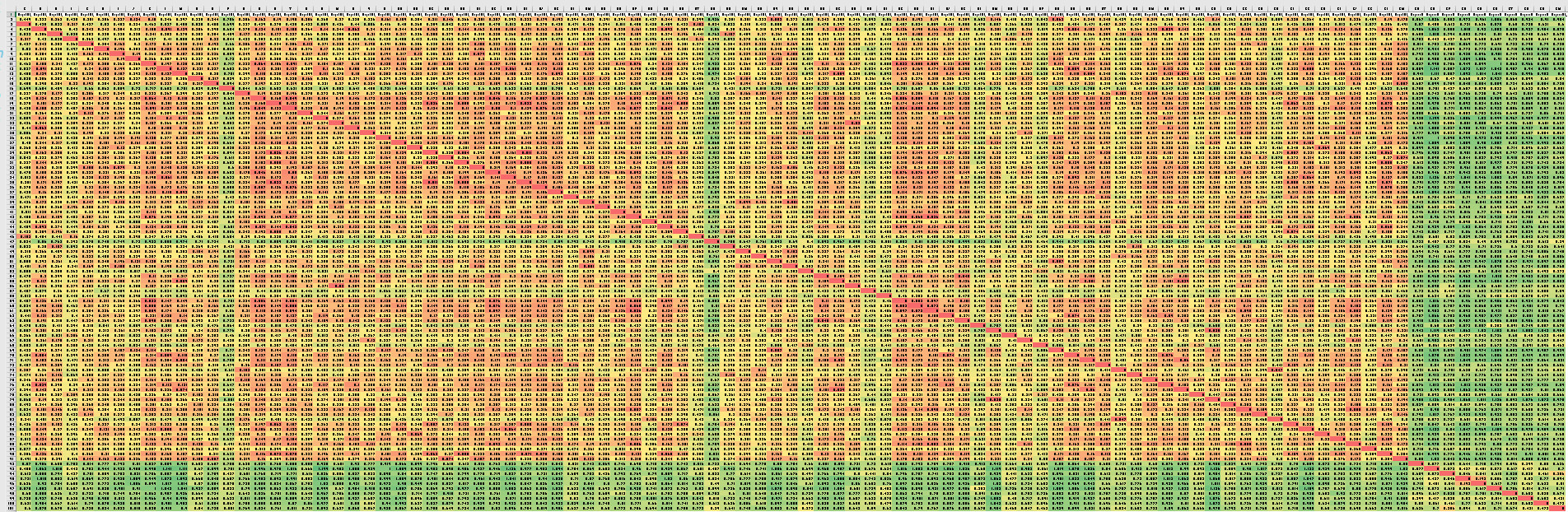
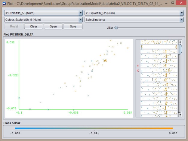
Although I can’t figure out how to classify using this data, clustering works pretty well. This is Canopy (WEKA) on the top dataset above:
=== Run information ===

Scheme: weka.clusterers.Canopy -N -1 -max-candidates 100 -periodic-pruning 10000 -min-density 2.0 -t2 -1.0 -t1 -1.25 -S 1
Relation: ORIGIN_POSITION_DELTA
Instances: 100
Attributes: 102
[list of attributes omitted]
Test mode: Classes to clusters evaluation on training data

=== Clustering model (full training set) ===

Canopy clustering
=================

Number of canopies (cluster centers) found: 2
T2 radius: 3.137
T1 radius: 3.922

Cluster 0: 0.283631,0.443357,0.240249,0.280277,0.396611,0.258673,0.28608,0.27558,0.312295,0.215801,0.249255,0.25779,0.280719,0.273191,0.58818,0.258901,0.196191,0.240405,0.201927,0.273491,0.271862,0.266807,0.249377,0.269756,0.265874,0.252873,0.299417,0.244208,0.284257,0.253868,0.234348,0.213578,0.242031,0.248292,0.215259,0.236993,0.301843,0.245444,0.282464,0.290885,0.216585,0.375846,0.223493,0.278251,0.375965,0.764462,0.338657,0.280672,0.316447,0.261622,0.265026,0.436098,0.246442,0.246887,0.289306,0.470806,0.43541,0.209845,0.220971,0.21506,0.247576,0.249173,0.468053,0.28907,0.418987,0.293851,0.452858,0.267638,0.243671,0.248868,0.242674,0.371534,0.29843,0.221506,0.25575,0.242182,0.335877,0.28386,0.303986,0.235298,0.282083,0.427425,0.26635,0.251009,0.304134,0.281157,0.212644,0.367693,0.222213,0.247862,0.780248,0.894699,0.713413,0.865287,0.826024,0.868741,0.757008,0.807287,0.785141,0.756071,{88}
Cluster 1: 0.919922,0.669721,0.908035,0.73578,0.591465,0.752733,0.774358,0.826861,0.84364,0.884803,0.939301,0.958981,0.629587,0.76459,0.545587,0.715267,0.853073,0.803545,0.851979,0.693952,0.954557,0.703606,0.897206,0.698297,0.926263,0.91898,0.733686,0.818759,0.763319,0.776199,0.843167,0.811708,0.903011,0.814435,0.804113,0.916336,0.639919,0.779399,0.663897,0.754696,0.77482,0.682512,0.832556,0.764008,0.703999,0.513612,0.693526,0.734279,0.723504,0.903016,0.777757,0.597915,0.86509,0.900357,0.724636,0.648915,0.577278,0.883327,0.828117,0.813873,0.860062,0.915821,0.684886,0.979451,0.556747,0.667678,0.556487,0.941671,0.898276,0.902846,0.686763,0.664381,0.709607,0.706246,0.890753,0.898794,0.588379,1.001214,0.625244,0.761188,0.828436,0.661864,0.759379,0.944355,0.728272,0.764909,0.761139,0.65028,0.845547,0.87213,0.586679,0.500194,0.498893,0.513267,0.493026,0.58192,0.620756,0.469854,0.540532,0.496272,{12}

Time taken to build model (full training data) : 0.03 seconds

=== Model and evaluation on training set ===

Clustered Instances

0 88 ( 88%)
1 12 ( 12%)

Class attribute: AgentBias_
Classes to Clusters:

0 1 -- assigned to cluster
0 10 | EXPLORER
88 2 | EXPLOITER

Cluster 0 -- EXPLOITER
Cluster 1 -- EXPLORER

Incorrectly clustered instances : 2.0 2 %
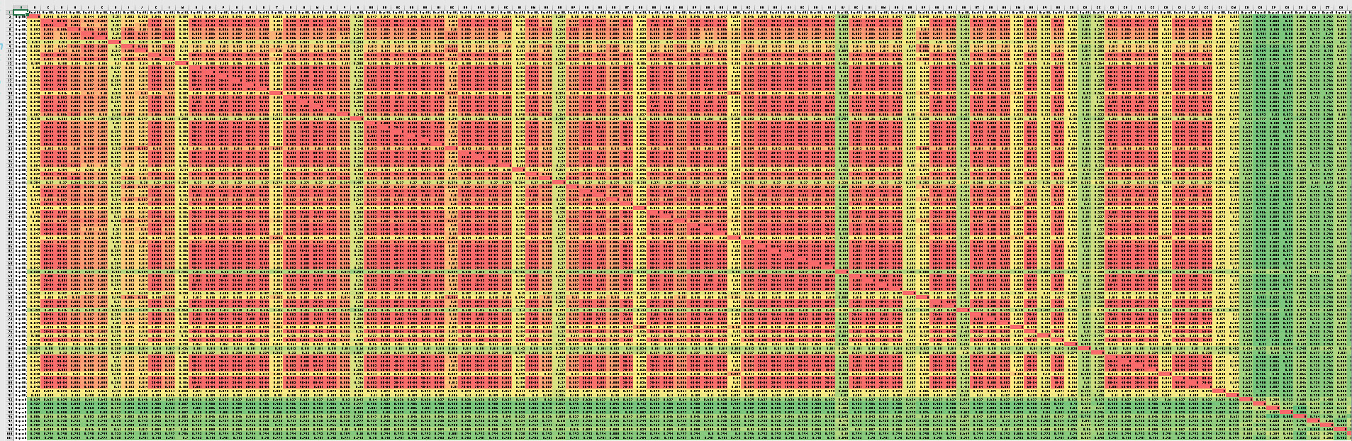
The next analyses is on the second dataset. They are essentially the same, even though the differences are more dramatic (the tight clusters are very tight
=== Run information ===

Scheme:       weka.clusterers.Canopy -N -1 -max-candidates 100 -periodic-pruning 10000 -min-density 2.0 -t2 -1.0 -t1 -1.25 -S 1
Relation:     ORIGIN_POSITION_DELTA
Instances:    100
Attributes:   102
              [list of attributes omitted]
Test mode:    Classes to clusters evaluation on training data

=== Clustering model (full training set) ===


Canopy clustering
=================

Number of canopies (cluster centers) found: 2
T2 radius: 3.438
T1 radius: 4.297

Cluster 0: 0.085848,0.050964,0.0513,0.053288,0.05439,0.054653,0.21758,0.057725,0.058775,0.050894,0.053768,0.130821,0.051098,0.050923,0.051115,0.050893,0.051012,0.051009,0.060649,0.051454,0.051089,0.051032,0.050894,0.053364,0.276684,0.051857,0.050984,0.050942,0.0509,0.050952,0.051025,0.056953,0.050914,0.050962,0.050903,0.052129,0.128196,0.051023,0.054222,0.274438,0.053978,0.050934,0.051124,0.054563,0.050995,0.074289,0.051077,0.05094,0.053644,0.050941,0.051343,0.050967,0.062704,0.052333,0.050936,0.051013,0.050922,0.051007,0.051038,0.050899,0.501239,0.051574,0.051005,0.050898,0.050944,0.204398,0.06076,0.050947,0.050904,0.408553,0.051263,0.0511,0.051574,0.069173,0.050997,0.162314,0.051353,0.096523,0.498648,0.339103,0.051125,0.050888,0.051002,0.051124,0.080711,0.05105,0.051024,0.050988,0.100492,0.132793,0.630178,0.882598,0.832132,0.86452,0.55151,0.729317,0.755526,0.513822,0.782104,0.768836,{92}
Cluster 1: 0.799117,0.793729,0.79643,0.7929,0.797843,0.797642,0.709935,0.78817,0.805937,0.794095,0.7972,0.76062,0.793743,0.79418,0.794846,0.794247,0.794677,0.793599,0.800359,0.794787,0.793849,0.793805,0.793613,0.784762,0.774656,0.79547,0.794308,0.793527,0.794406,0.793292,0.793513,0.800151,0.793775,0.793652,0.794123,0.793645,0.73331,0.794506,0.788542,0.710244,0.793332,0.793313,0.794184,0.801119,0.79448,0.802416,0.793669,0.7947,0.794813,0.794533,0.796484,0.794512,0.797614,0.794607,0.793716,0.793642,0.793548,0.794789,0.793551,0.793989,0.539133,0.79391,0.793443,0.793969,0.794472,0.715896,0.790956,0.794494,0.794293,0.678147,0.79434,0.793611,0.794221,0.802197,0.793753,0.759132,0.794164,0.798071,0.55929,0.698333,0.79444,0.79424,0.793585,0.793581,0.779958,0.79394,0.793567,0.794795,0.764686,0.754727,0.482214,0.518683,0.434538,0.501648,0.790616,0.4855,0.464554,0.691735,0.405411,0.496892,{8}


Time taken to build model (full training data) : 0.01 seconds

=== Model and evaluation on training set ===

Clustered Instances

0       88 ( 88%)
1       12 ( 12%)


Class attribute: AgentBias_
Classes to Clusters:

  0  1  -- assigned to cluster
  0 10 | EXPLORER
 88  2 | EXPLOITER

Cluster 0 -- EXPLOITER
Cluster 1 -- EXPLORER

Incorrectly clustered instances :	2.0	  2      %


 Exploit-Exploit
  Explore-Exploit
 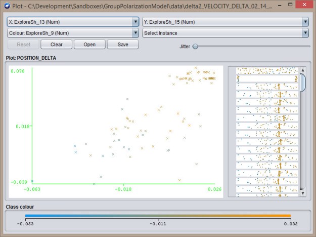 Explore-Explore


You must be logged in to post a comment.