Transformer Architecture: The Positional Encoding

• In this article, I don’t plan to explain its architecture in depth as there are currently several great tutorials on this topic (here, here, and here), but alternatively, I want to discuss one specific part of the transformer’s architecture – the positional encoding.

D20

• Add centroids for states – done
• Return the number of neighbors as an argument – done
• Chatted with Aaron and Zach. More desire to continue than abandon

ACSOS

• More revisions. Swap steps for discussion and future work

GOES

• • IRS proposal went in yesterday
  • Continue with GANs
  • Using the VGG model now with much better results. Also figured out how to loads weights and read the probabilities in the output layer:
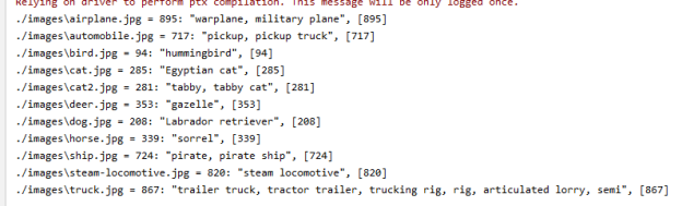
  • Same thing using the pre-trained model from Keras:

    from tensorflow.keras.applications.vgg16 import VGG16
    # prebuild model with pre-trained weights on imagenet
    model = VGG16(weights='imagenet', include_top=True)
    model.compile(optimizer='sgd', loss='categorical_crossentropy')

    

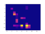
  • Trying to visualize a layer using this code. And using that code as a starting point, I had to explore how to slice up the tensors in the right way. A CNN layer has a set of “filters” that contain a square set of pixels. The data is stored as an array of pixels at each x, y, coordinate, so I had to figure out how to get one image at a time. Here’s my toy:

    import numpy as np
    import matplotlib.pyplot as plt
    
    n_rows = 4
    n_cols = 8
    depth = 4
    
    my_list = []
    
    for r in range(1, n_rows):
        row = []
        my_list.append(row)
        for c in range(1, n_cols):
            cell = []
            row.append(cell)
            for d in range(depth):
                cell.append(d+c*10+r*100)
    
    print(my_list)
    nl = np.array(my_list)
    for d in range(depth):
        print("\nlayer {} = \n{}".format(d, nl[:, :, d]))
        plt.figure(d)
        plt.imshow(nl[:, :, d], aspect='auto', cmap='plasma')
    
    plt.show()

  • This gets features from a cat image at one of the pooling layers. The color map is completely arbitrary:

    # get the features from this block
    features = model.predict(x)
    print(features.shape)
    farray = np.array(features[0])
    print("{}".format(farray[:, :, 0]))
    
    for d in range(4):
       plt.figure(d)
       plt.imshow(farray[:, :, d], aspect='auto', cmap='plasma')

  • But we get some cool pix!